2026-10-06 · 微积分与优化

高级工程数学

2026-10-06

沈超敏

计算机科学与技术学院

cmshen@cs.ecnu.edu.cn

文附楼 105

复习

Ch. 3. Transformations
3.1 Linear Transformations
3.2 Eigenvalues and Eigenvectors
3.3 Orthogonal Projections
3.4 Quadratic Forms
3.5 Matrix Norms 3.5 Exercises

上次课例题

习题3.5 对 \(A = \begin{bmatrix} -1 & 0 & 0 & 0 \\ 1 & 1 & 0 & 0 \\ 2 & 5 & 2 & 1 \\ -1 & 1 & 0 & 3 \end{bmatrix}\) 给出的linear transform, 找一组基, 使在这组基下A对应的矩阵是对角阵.

解: 该题意思是: A 代表一个变换, 将 x 变成 y, 即 Ax = y (这里 A 就是变换对应的矩阵, A, x, y, 均在自然基下表示).

该题问，如果换了一组基，在新基下 A 对应的矩阵如记成 B，要使 B 是对角阵，基应如何取法.

Claim: 新基取 A 的一组特征向量 \(\{v_1,\ldots,v_n\}\)（若它们构成一组基），则新基下 A 的矩阵为 \(\Lambda=\operatorname{diag}(\lambda_1,\ldots,\lambda_n)\)。

理由: x 在 \(\{e_{1},\cdots,e_{n}\}\) 下的坐标是 \(\begin{bmatrix}x_{1}\\ \vdots\\ x_{n}\end{bmatrix}\) ，在 \(\{v_{1},\cdots,v_{n}\}\) 下坐标 \(\begin{bmatrix}a_{1}\\ \vdots\\ a_{n}\end{bmatrix}\) . y 在 \(\{e_{1},\cdots,e_{n}\}\) 下的坐标是 \(\begin{bmatrix}y_{1}\\ \vdots\\ y_{n}\end{bmatrix}\) ，在 \(\{v_{1},\cdots,v_{n}\}\) 下坐标 \(\begin{bmatrix}b_{1}\\ \vdots\\ b_{n}\end{bmatrix}\) . 令 \(V=[v_1\ \cdots\ v_n]\)，则

\[x=Va,\qquad y=Vb.\tag{1–2}\]

对 (1) 两端左乘 \(\vec{A}\) , 得

\[AVa=V\Lambda a,\]

而 \(A\left[\begin{array}{c}x_{1}\\ \vdots\\ x_{n}\end{array}\right]=y=V\left[\begin{array}{c}b_{1}\\ \vdots\\ b_{n}\end{array}\right]\) (由（2）式可得).

所以，

\[V\Lambda a=Vb,\qquad b=\Lambda a. \]

因此，在基 \(V\) 下，A 的矩阵表示为对角矩阵 \(\Lambda\)。

上次补充例题

\(\overrightarrow{x}\) , 经正交变换 \((Q^T Q = I)\) , 变成 \(\overrightarrow{y}\) ,

问 \(\overrightarrow{y}\) 的长度和 \(\overrightarrow{x}\) 的长度的关系。

答：由 \(\overrightarrow{y}=Q\overrightarrow{x}\)，其长度可通过内积计算：

\(\langle Q\overrightarrow{x},Q\overrightarrow{x}\rangle=(Q\overrightarrow{x})^{T}Q\overrightarrow{x}=\overrightarrow{x}^{T}Q^{T}Q\overrightarrow{x}\)

3.4 Quadratic Forms

A quadratic form \(f:\mathbb{R}^{n}\to\mathbb{R}\) is a function

\[ f (\boldsymbol {x}) = \boldsymbol {x} ^ {\top} Q \boldsymbol {x}, \]

where Q is an \(n \times n\) real matrix.

假设 Q 是对称的.

称 quadratic form \(x^{\top}Qx\) 是 positive definite, if \(x^{\top}Qx > 0\) for all nonzero x. Semidefinite if \(x^{\top}Qx \geq 0\) for all nonzero x.

The analogous notions are negative definite and negative semidefinite.

3.5 Matrix Norms

Using arguments similar to the above, we can deduce the following important inequalities.

Rayleigh's Inequalities. If an \(n \times n\) matrix \(P\) is real symmetric positive definite, then

\[ \lambda_ {\min} (\boldsymbol {P}) \| \boldsymbol {x} \| ^ {2} \leq \boldsymbol {x} ^ {\top} \boldsymbol {P} \boldsymbol {x} \leq \lambda_ {\max} (\boldsymbol {P}) \| \boldsymbol {x} \| ^ {2}, \]

where \(\lambda_{\min}(\boldsymbol{P})\) denotes the smallest eigenvalue of P, and \(\lambda_{\max}(\boldsymbol{P})\) denotes the largest eigenvalue of P.

Concepts from Geometry 4.1 Line Segments 4.2 Hyperplanes and Linear Varieties 4.3 Convex Sets 4.4 Neighborhoods 4.5 Polytopes and Polyhedra

第四章内容总结

超平面是 n-1 维的, 因为 \(x_{1}, \cdots, x_{n}\) 是 n 维的, 超平面给了一个限制条件, 所以有 n-1 个自由度.

超平面法线的理解：法线先记作 \(n\) (normal 的意思), normal 应满足同超平面内任意向量垂直, 那如何表示超平面内任何向量呢？超平面内找一个已知点 \(a\) , 再找任意点 \(x\) , 则 \(x - a\) 可代表超平面内任意向量, slide 中已证 \(\langle u, a - x \rangle = 0\) , 所以 \(u\) 即所求的法线.

超平面的交可以这样理解：每个方程都可写成 \(a_1x_1 + \ldots + a_nx_n = b\)，对应一个超平面，所以方程组的解是这些超平面的交。方程数不一定等于不同超平面的个数，因为方程可能重复。

凸集概念在后面带限制条件的优化问题要用到, 直观上说, 优化迭代时, \(x_{1}\) 跳到 \(x_{2}, x_{2}\) 跳到 \(x_{3}\) , 我至少要保证点都在规定的集合中. 跳的时候还有跳多远 (步长) 的事, 如果两点间所有的点都在集合中, 可以根据需要, 有时跳近点.

今天: Elements of Calculus 5.1 Sequences and Limits 5.2 Differentiability 5.3 The Derivative Matrix 5.4 Differentiation Rules 5.5 Level Sets and Gradients 5.6 Taylor Series

5.1 Sequences and Limits

A sequence of real numbers is a function whose domain is the set of natural numbers \(1,2,\ldots,k,\ldots\) and whose range is contained in R. Thus, a sequence of real numbers can be viewed as a set of numbers \(\{x_{1},x_{2},\ldots,x_{k},\ldots\}\) , which is often also denoted as \(\{x_{k}\}\) (or sometimes as \(\{x_{k}\}_{k=1}^{\infty}\) , to indicate explicitly the range of values that k can take).

A sequence \(\{x_{k}\}\) is increasing if \(x_{1}<x_{2}<\cdots<x_{k}\cdots\) ; that is, \(x_{k}<x_{k+1}\) for all k. If \(x_{k}\leq x_{k+1}\) , then we say that the sequence is nondecreasing. Similarly, we can define decreasing and nonincreasing sequences. Nonincreasing or nondecreasing sequences are called monotone sequences.

A number \(x^{*} \in R\) is called the limit of the sequence \(\{x_{k}\}\) if for any positive \(\varepsilon\) there is a number K (which may depend on \(\varepsilon\) ) such that for all k > K, \(|x_{k} - x^{*}| < \varepsilon\) ; that is, \(x_{k}\) lies between \(x^{*} - \varepsilon\) and \(x^{*} + \varepsilon\) for all k > K. In this case we write

\[ x ^ {*} = \lim _ {k \rightarrow \infty} x _ {k} \]

or

\[ x _ {k} \rightarrow x ^ {*}. \]

5.1 Sequences and Limits ( \(R^{n}\) )

The notion of a sequence can be extended to sequences with elements in \(\mathbb{R}^n\) . Specifically, a sequence in \(\mathbb{R}^n\) is a function whose domain is the set of natural numbers \(1,2,\ldots,k,\ldots\) and whose range is contained in \(\mathbb{R}^n\) . We use the notation \(\{\pmb{x}^{(1)},\pmb{x}^{(2)},\dots\}\) or \(\{\pmb{x}^{(k)}\}\) for sequences in \(\mathbb{R}^n\) . For limits of sequences in \(\mathbb{R}^n\) , we need to replace absolute values with vector norms. In other words, \(\pmb{x}^*\) is the limit of \(\{\pmb{x}^{(k)}\}\) if for any positive \(\varepsilon\) there is a number \(K\) (which may depend on \(\varepsilon\) ) such that for all \(k > K\) , \(\| \pmb{x}^{(k)} - \pmb{x}^* \| < \varepsilon\) . As before, if a sequence \(\{\pmb{x}^{(k)}\}\) is convergent, we write \(\pmb{x}^* = \lim_{k\to \infty}\pmb{x}^{(k)}\) or \(\pmb{x}^{(k)}\to \pmb{x}^*\) .

5.1 Sequences and Limits (唯一性)

Theorem 5.1 A convergent sequence has only one limit.

Proof. We prove this result by contradiction. Suppose that a sequence \(\{\pmb{x}^{(k)}\}\) has two different limits, say \(\pmb{x}_1\) and \(\pmb{x}_2\) . Then, we have \(\| \pmb{x}_1 - \pmb{x}_2 \| > 0\) . Let

\[ \varepsilon = \frac {1}{2} \| \boldsymbol {x} _ {1} - \boldsymbol {x} _ {2} \|. \]

From the definition of a limit, there exist \(K_{1}\) and \(K_{2}\) such that for \(k > K_{1}\) we have \(\| \pmb{x}^{(k)} - \pmb{x}_1 \| < \varepsilon\) , and for \(k > K_{2}\) we have \(\| \pmb{x}^{(k)} - \pmb{x}_2 \| < \varepsilon\) . Let \(K = \max \{K_1, K_2\}\) . Then, if \(k > K\) , we have \(\| \pmb{x}^{(k)} - \pmb{x}_1 \| < \varepsilon\) and \(\| \pmb{x}^{(k)} - \pmb{x}_2 \| < \varepsilon\) . Adding \(\| \pmb{x}^{(k)} - \pmb{x}_1 \| < \varepsilon\) and \(\| \pmb{x}^{(k)} - \pmb{x}_2 \| < \varepsilon\) yields

\[ \left\| \boldsymbol {x} ^ {(k)} - \boldsymbol {x} _ {1} \right\| + \left\| \boldsymbol {x} ^ {(k)} - \boldsymbol {x} _ {2} \right\| < 2 \varepsilon . \]

Applying the triangle inequality gives

\[ \begin{array}{r l} \| - \boldsymbol {x} _ {1} + \boldsymbol {x} _ {2} \| & = \| \boldsymbol {x} ^ {(k)} - \boldsymbol {x} _ {1} - \boldsymbol {x} ^ {(k)} + \boldsymbol {x} _ {2} \| \\ & = \| (\boldsymbol {x} ^ {(k)} - \boldsymbol {x} _ {1}) - (\boldsymbol {x} ^ {(k)} - \boldsymbol {x} _ {2}) \| \\ & \leq \| \boldsymbol {x} ^ {(k)} - \boldsymbol {x} _ {1} \| + \| \boldsymbol {x} ^ {(k)} - \boldsymbol {x} _ {2} \|. \end{array} \]

Therefore,

\[ \| - \boldsymbol {x} _ {1} + \boldsymbol {x} _ {2} \| = \| \boldsymbol {x} _ {1} - \boldsymbol {x} _ {2} \| < 2 \varepsilon . \]

However, this contradicts the assumption that \(\|x_{1}-x_{2}\|=2\varepsilon\) , which completes the proof.

5.1 Sequences and Limits (有界性)

A sequence \(\{\pmb{x}^{(k)}\}\) in \(\mathbb{R}^n\) is bounded if there exists a number \(B \geq 0\) such that \(\| \pmb{x}^{(k)} \| \leq B\) for all \(k = 1,2,\ldots\) .

Theorem 5.2 Every convergent sequence is bounded.

Proof. Let \(\{\pmb{x}^{(k)}\}\) be a convergent sequence with limit \(\pmb{x}^*\) . Choose \(\varepsilon = 1\) . Then, by definition of the limit, there exists a natural number \(K\) such that for all \(k > K\) ,

\[ \left\| \boldsymbol {x} ^ {(k)} - \boldsymbol {x} ^ {*} \right\| < 1. \]

By the result of Exercise 2.9, we get

\[ \| \boldsymbol {x} ^ {(k)} \| - \| \boldsymbol {x} ^ {*} \| \leq \| \boldsymbol {x} ^ {(k)} - \boldsymbol {x} ^ {*} \| < 1 \quad \text { for all } k > K. \]

Therefore,

\[ \| \boldsymbol {x} ^ {(k)} \| < \| \boldsymbol {x} ^ {*} \| + 1 \quad \text { for all } k > K. \]

Letting

\[ B = \max \left\{\| \boldsymbol {x} ^ {(1)} \|, \| \boldsymbol {x} ^ {(2)} \|, \dots , \| \boldsymbol {x} ^ {(K)} \|, \| \boldsymbol {x} ^ {*} \| + 1 \right\}, \]

we have

\[ B \geq \| \boldsymbol {x} ^ {(k)} \| \quad \text { for all } k, \]

which means that the sequence \(\{\pmb{x}^{(k)}\}\) is bounded.

5.1 Sequences and Limits (上确界)

For a sequence \(\{x_{k}\}\) in R, a number B is called an upper bound if \(x_{k} \leq B\) for all \(k = 1, 2, \ldots\) . In this case, we say that \(\{x_{k}\}\) is bounded above. Similarly, B is called a lower bound if \(x_{k} \geq B\) for all \(k = 1, 2, \ldots\) . In this case, we say that \(\{x_{k}\}\) is bounded below. Clearly, a sequence is bounded if it is both bounded above and bounded below.

Any sequence \(\{x_{k}\}\) in R that has an upper bound has a least upper bound (also called the supremum), which is the smallest number B that is an upper bound of \(\{x_{k}\}\) . Similarly, any sequence \(\{x_{k}\}\) in R that has a lower bound has a greatest lower bound (also called the infimum). If B is the least upper bound of the sequence \(\{x_{k}\}\) , then \(x_{k} \leq B\) for all k, and for any \(\varepsilon > 0\) , there exists a number K such that \(x_{K} > B - \varepsilon\) . An analogous statement applies to the greatest lower bound: If B is the greatest lower bound of \(\{x_{k}\}\) , then \(x_{k} \geq B\) for all k, and for any \(\varepsilon > 0\) , there exists a number K such that \(x_{K} < B + \varepsilon\) .

5.1 Sequences and Limits （单调有界必收敛）

Theorem 5.3 Every monotone bounded sequence in \(\mathbb{R}\) is convergent.

Proof. We prove the theorem for nondecreasing sequences. The proof for nonincreasing sequences is analogous.

Let \(\{x_{k}\}\) be a bounded nondecreasing sequence in \(\mathbb{R}\) and \(x^{*}\) the least upper bound. Fix a number \(\varepsilon > 0\) . Then, there exists a number \(K\) such that \(x_{K} > x^{*} - \varepsilon\) . Because \(\{x_{k}\}\) is nondecreasing, for any \(k \geq K\) ,

\[ x _ {k} \geq x _ {K} > x ^ {*} - \varepsilon . \]

Also, because \(x^{*}\) is an upper bound of \(\{x_{k}\}\) , we have

\[ x _ {k} \leq x ^ {*} < x ^ {*} + \varepsilon . \]

Therefore, for any \(k \geq K\) ,

\[ \left| x _ {k} - x ^ {*} \right| < \varepsilon , \]

which means that \(x_{k} \rightarrow x^{*}\) .

5.1 Sequences and Limits （收敛序列的子序列必收敛）

Theorem 5.4 Consider a convergent sequence \(\{\pmb{x}^{(k)}\}\) with limit \(\pmb{x}^*\) . Then, any subsequence of \(\{\pmb{x}^{(k)}\}\) also converges to \(\pmb{x}^*\) .

Proof. Let \(\{\pmb{x}^{(m_k)}\}\) be a subsequence of \(\{\pmb{x}^{(k)}\}\) , where \(\{m_k\}\) is an increasing sequence of natural numbers. Observe that \(m_k \geq k\) for all \(k = 1,2,\ldots\) . To show this, first note that \(m_1 \geq 1\) because \(m_1\) is a natural number. Next, we proceed by induction by assuming that \(m_k \geq k\) . Then, we have \(m_{k+1} > m_k \geq k\) , which implies that \(m_{k+1} \geq k + 1\) . Therefore, we have shown that \(m_k \geq k\) for all \(k = 1,2,\ldots\) .

Let \(\varepsilon > 0\) be given. Then, by definition of the limit, there exists \(K\) such that \(\| \pmb{x}^{(k)} - \pmb{x}^* \| < \varepsilon\) for any \(k > K\) . Because \(m_k \geq k\) , we also have \(\| \pmb{x}^{(m_k)} - \pmb{x}^* \| < \varepsilon\) for any \(k > K\) . This means that

\[ \lim _ {k \rightarrow \infty} \boldsymbol {x} ^ {(m _ {k})} = \boldsymbol {x} ^ {*}. \]

It turns out that any bounded sequence contains a convergent subsequence. This result is called the Bolzano-Weierstrass theorem (see [2, p. 70]).

5.1 Sequences and Limits (连续)

Consider a function \(\pmb{f}:\mathbb{R}^n\to \mathbb{R}^m\) and a point \(\pmb{x}_0\in \mathbb{R}^n\) . Suppose that there exists \(f^{*}\) such that for any convergent sequence \(\{\pmb{x}^{(k)}\}\) with limit \(\pmb{x}_0\) , we have

\[ \lim _ {k \rightarrow \infty} \boldsymbol {f} (\boldsymbol {x} ^ {(k)}) = \boldsymbol {f} ^ {*}. \]

Then, we use the notation

\[ \lim _ {\boldsymbol {x} \rightarrow \boldsymbol {x} _ {0}} \boldsymbol {f} (\boldsymbol {x}) \]

to represent the limit \(f^{*}\) .

It turns out that f is continuous at \(x_{0}\) if and only if for any convergent sequence \(\{\boldsymbol{x}^{(k)}\}\) with limit \(x_{0}\) , we have

\[ \lim _ {k \rightarrow \infty} f (x ^ {(k)}) = f \left(\lim _ {k \rightarrow \infty} x ^ {(k)}\right) = f (x _ {0}) \]

(see [2, p. 137]). Therefore, using the notation introduced above, the function \(\pmb{f}\) is continuous at \(x_0\) if and only if

\[ \lim _ {\boldsymbol {x} \rightarrow \boldsymbol {x} _ {0}} \boldsymbol {f} (\boldsymbol {x}) = \boldsymbol {f} (\boldsymbol {x} _ {0}). \]

5.1 Sequences and Limits

矩阵的极限

We say that a sequence \(\{\pmb{A}_k\}\) of \(m \times n\) matrices converges to the \(m \times n\) matrix \(\pmb{A}\) if

\[ \lim _ {k \rightarrow \infty} \| \boldsymbol {A} - \boldsymbol {A} _ {k} \| = 0. \]

Lemma 5.1 Let \(\mathbf{A} \in \mathbb{R}^{n \times n}\) . Then, \(\lim_{k \to \infty} \mathbf{A}^k = \mathbf{O}\) if and only if the eigenvalues of \(\mathbf{A}\) satisfy \(|\lambda_i(\mathbf{A})| < 1\) , \(i = 1, \ldots, n\) .

5.2 Differentiability

Differential calculus is based on the idea of approximating an arbitrary function by an affine function. A function \(\mathcal{A}:\mathbb{R}^{n}\to\mathbb{R}^{m}\) is affine if there exists a linear function \(\mathcal{L}:\mathbb{R}^{n}\to\mathbb{R}^{m}\) and a vector \(y\in\mathbb{R}^{m}\) such that

\[ \mathcal {A} (\boldsymbol {x}) = \mathcal {L} (\boldsymbol {x}) + \boldsymbol {y} \]

for every \(x \in R^{n}\) . Consider a function \(f : R^{n} \to R^{m}\) and a point \(x_{0} \in R^{n}\) . We wish to find an affine function A that approximates f near the point \(x_{0}\) . First, it is natural to impose the condition

\[ \mathcal {A} (\boldsymbol {x} _ {0}) = \boldsymbol {f} (\boldsymbol {x} _ {0}). \]

Because \(\mathcal{A}(\pmb{x}) = \mathcal{L}(\pmb{x}) + \pmb{y}\) , we obtain \(\pmb{y} = \pmb{f}(\pmb{x}_0) - \mathcal{L}(\pmb{x}_0)\) . By the linearity of \(\mathcal{L}\) ,

\[ \mathcal {L} (\boldsymbol {x}) + \boldsymbol {y} = \mathcal {L} (\boldsymbol {x}) - \mathcal {L} (\boldsymbol {x} _ {0}) + \boldsymbol {f} (\boldsymbol {x} _ {0}) = \mathcal {L} (\boldsymbol {x} - \boldsymbol {x} _ {0}) + \boldsymbol {f} (\boldsymbol {x} _ {0}). \]

Hence, we may write

\[ \mathcal {A} (\boldsymbol {x}) = \mathcal {L} (\boldsymbol {x} - \boldsymbol {x} _ {0}) + \boldsymbol {f} (\boldsymbol {x} _ {0}). \]

Next, we require that \(\mathcal{A}(\pmb{x})\) approaches \(\pmb{f}(\pmb{x})\) faster than \(\pmb{x}\) approaches \(\pmb{x}_0\) ; that is,

\[ \lim _ {\boldsymbol {x} \rightarrow \boldsymbol {x} _ {0}, \boldsymbol {x} \in \Omega} \frac {\| \boldsymbol {f} (\boldsymbol {x}) - \mathcal {A} (\boldsymbol {x}) \|}{\| \boldsymbol {x} - \boldsymbol {x} _ {0} \|} = 0. \]

The conditions above on A ensure that A approximates f near \(x_{0}\) in the sense that the error in the approximation at a given point is “small” compared with the distance of the point from \(x_{0}\) .

5.3 The Derivative Matrix

Any linear transformation from \(\mathbb{R}^n\) to \(\mathbb{R}^m\) , and in particular the derivative \(\mathcal{L}\) of \(f: \mathbb{R}^n \to \mathbb{R}^m\) , can be represented by an \(m \times n\) matrix. To find the matrix representation \(L\) of the derivative \(\mathcal{L}\) of a differentiable function \(f: \mathbb{R}^n \to \mathbb{R}^m\) , we use the natural basis \(\{e_1, \ldots, e_n\}\) for \(\mathbb{R}^n\) . Consider the vectors

\[ \boldsymbol {x} _ {j} = \boldsymbol {x} _ {0} + t \boldsymbol {e} _ {j}, \quad j = 1, \dots , n. \]

By the definition of the derivative, we have

\[ \lim _ {t \rightarrow 0} \frac {\boldsymbol {f} (\boldsymbol {x} _ {j}) - (t \boldsymbol {L e} _ {j} + \boldsymbol {f} (\boldsymbol {x} _ {0}))}{t} = \mathbf {0} \]

for \(j = 1, \ldots, n\) . This means that

\[ \lim _ {t \rightarrow 0} \frac {\boldsymbol {f} (\boldsymbol {x} _ {j}) - \boldsymbol {f} (\boldsymbol {x} _ {0})}{t} = \boldsymbol {L e} _ {j} \]

for \(j = 1, \ldots, n\) . But \(Le_{j}\) is the jth column of the matrix L. On the other hand, the vector \(x_{j}\) differs from \(x_{0}\) only in the jth coordinate, and in that coordinate the difference is just the number t. Therefore, the left side of the preceding equation is the partial derivative

\[ \frac {\partial \boldsymbol {f}}{\partial x _ {j}} (\boldsymbol {x} _ {0}). \]

Because vector limits are computed by taking the limit of each coordinate function, it follows that if

\[ \boldsymbol {f} (\boldsymbol {x}) = \left[ \begin{array}{c} f _ {1} (\boldsymbol {x}) \\ \vdots \\ f _ {m} (\boldsymbol {x}) \end{array} \right], \]

then

\[ \frac {\partial \boldsymbol {f}}{\partial x _ {j}} (\boldsymbol {x} _ {0}) = \left[ \begin{array}{c} \frac {\partial f _ {1}}{\partial x _ {j}} (\boldsymbol {x} _ {0}) \\ \vdots \\ \frac {\partial f _ {m}}{\partial x _ {j}} (\boldsymbol {x} _ {0}) \end{array} \right], \]

Theorem 5.5 If a function \(\pmb{f} : \mathbb{R}^n \to \mathbb{R}^m\) is differentiable at \(x_0\) , then the derivative of \(\pmb{f}\) at \(x_0\) is determined uniquely and is represented by the \(m \times n\) derivative matrix \(D\pmb{f}(x_0)\) . The best affine approximation to \(\pmb{f}\) near \(x_0\) is then given by

\[ \mathcal {A} (\boldsymbol {x}) = \boldsymbol {f} \left(\boldsymbol {x} _ {0}\right) + D \boldsymbol {f} \left(\boldsymbol {x} _ {0}\right) \left(\boldsymbol {x} - \boldsymbol {x} _ {0}\right), \]

in the sense that

\[ \boldsymbol {f} (\boldsymbol {x}) = \mathcal {A} (\boldsymbol {x}) + \boldsymbol {r} (\boldsymbol {x}) \]

and \(\lim_{x\to x_{0}}\|r(x)\|/\|x-x_{0}\|=0\) . The columns of the derivative matrix \(Df(x_{0})\) are vector partial derivatives. The vector

\[ \frac {\partial \boldsymbol {f}}{\partial x _ {j}} (\boldsymbol {x} _ {0}) \]

is a tangent vector at \(x_{0}\) to the curve f obtained by varying only the jth coordinate of x. □

If \(f:\mathbb{R}^{n}\to \mathbb{R}\) is differentiable, then the function \(\nabla f\) defined by

\[ \nabla f (\boldsymbol {x}) = \left[ \begin{array}{c} \frac {\partial f}{\partial x _ {1}} (\boldsymbol {x}) \\ \vdots \\ \frac {\partial f}{\partial x _ {n}} (\boldsymbol {x}) \end{array} \right] = D f (\boldsymbol {x}) ^ {\top} \]

is called the gradient of \(f\) . The gradient is a function from \(\mathbb{R}^n\) to \(\mathbb{R}^n\) , and can be pictured as a vector field, by drawing the arrow representing \(\nabla f(\pmb{x})\) so that its tail starts at \(\pmb{x}\) .

Given \(f: \mathbb{R}^n \to \mathbb{R}\) , if \(\nabla f\) is differentiable, we say that \(f\) is twice differentiable, and we write the derivative of \(\nabla f\) as

\[ D ^ {2} f = \left[ \begin{array}{c c c c} \frac {\partial^ {2} f}{\partial x _ {1} ^ {2}} & \frac {\partial^ {2} f}{\partial x _ {2} \partial x _ {1}} & \dots & \frac {\partial^ {2} f}{\partial x _ {n} \partial x _ {1}} \\ \frac {\partial^ {2} f}{\partial x _ {1} \partial x _ {2}} & \frac {\partial^ {2} f}{\partial x _ {2} ^ {2}} & \dots & \frac {\partial^ {2} f}{\partial x _ {n} \partial x _ {2}} \\ \vdots & \vdots & \ddots & \vdots \\ \frac {\partial^ {2} f}{\partial x _ {1} \partial x _ {n}} & \frac {\partial^ {2} f}{\partial x _ {2} \partial x _ {n}} & \dots & \frac {\partial^ {2} f}{\partial x _ {n} ^ {2}} \end{array} \right]. \]

(The notation \(\frac{\partial^2f}{\partial x_i\partial x_j}\) represents taking the partial derivative of \(f\) with respect to \(x_{j}\) first, then with respect to \(x_{i}\) .) The matrix \(D^2 f(\pmb {x})\) is called the Hessian matrix of \(f\) at \(\pmb{x}\) , and is often also denoted \(\pmb{F}(\pmb{x})\) .

Note that the Hessian matrix of a function \(f: R^{n} \to R\) at x is symmetric if f is twice continuously differentiable at x. This is a well-known result from calculus called Clairaut's theorem or Schwarz's theorem. However, if the second partial derivatives of f are not continuous, then there is no guarantee that the Hessian is symmetric, as shown in the following well-known example.

Example 5.1 Consider the function

\[ f (\boldsymbol {x}) = \left\{ \begin{array}{l l} x _ {1} x _ {2} (x _ {1} ^ {2} - x _ {2} ^ {2}) / (x _ {1} ^ {2} + x _ {2} ^ {2}) & \text { if } \boldsymbol {x} \neq \boldsymbol {0} \\ 0 & \text { if } \boldsymbol {x} = \boldsymbol {0}. \end{array} \right. \]

5.4 Differentiation Rules

We now introduce the chain rule for differentiating the composition \(g(\boldsymbol{f}(t))\) , of a function \(f: R \to R^{n}\) and a function \(g: R^{n} \to R\) .

Theorem 5.6 Let \(g: \mathcal{D} \to \mathbb{R}\) be differentiable on an open set \(\mathcal{D} \subset \mathbb{R}^n\) , and let \(f: (a, b) \to \mathcal{D}\) be differentiable on \((a, b)\) . Then, the composite function \(h: (a, b) \to \mathbb{R}\) given by \(h(t) = g(f(t))\) is differentiable on \((a, b)\) , and

\[ h ^ {\prime} (t) = D g (\boldsymbol {f} (t)) D \boldsymbol {f} (t) = \nabla g (\boldsymbol {f} (t)) ^ {\top} \left[ \begin{array}{c} f _ {1} ^ {\prime} (t) \\ \vdots \\ f _ {n} ^ {\prime} (t) \end{array} \right]. \]

Proof. By definition,

\[ h ^ {\prime} (t) = \lim _ {s \rightarrow t} \frac {h (s) - h (t)}{s - t} = \lim _ {s \rightarrow t} \frac {g (\boldsymbol {f} (s)) - g (\boldsymbol {f} (t))}{s - t} \]

if the limit exists. By Theorem 5.5 we write

\[ g (\boldsymbol {f} (s)) - g (\boldsymbol {f} (t)) = D g (\boldsymbol {f} (t)) (\boldsymbol {f} (s) - \boldsymbol {f} (t)) + r (s), \]

where \(\lim_{s\to t}r(s)/(s-t)=0\) . Therefore,

\[ \frac {h (s) - h (t)}{s - t} = D g (\boldsymbol {f} (t)) \frac {\boldsymbol {f} (s) - \boldsymbol {f} (t)}{s - t} + \frac {r (s)}{s - t}. \]

Letting \(s\to t\) yields

\[ h ^ {\prime} (t) = \lim _ {s \rightarrow t} D g (\boldsymbol {f} (t)) \frac {\boldsymbol {f} (s) - \boldsymbol {f} (t)}{s - t} + \frac {r (s)}{s - t} = D g (\boldsymbol {f} (t)) D \boldsymbol {f} (t). \]

Next, we present the product rule. Let \(\pmb{f}:\mathbb{R}^n\to \mathbb{R}^m\) and \(\pmb {g}:\mathbb{R}^n\to \mathbb{R}^m\) be two differentiable functions. Define the function \(h:\mathbb{R}^n\to \mathbb{R}\) by \(h(\pmb {x}) = \pmb {f}(\pmb {x})^{\top}\pmb {g}(\pmb {x})\) . Then, \(h\) is also differentiable and

\[ D h (\boldsymbol {x}) = \boldsymbol {f} (\boldsymbol {x}) ^ {\top} D \boldsymbol {g} (\boldsymbol {x}) + \boldsymbol {g} (\boldsymbol {x}) ^ {\top} D \boldsymbol {f} (\boldsymbol {x}). \]

We end this section with a list of some useful formulas from multivariable calculus. In each case, we compute the derivative with respect to x. Let \(A \in R^{m \times n}\) be a given matrix and \(y \in R^{m}\) a given vector. Then,

\[ \begin{array}{l} D (\boldsymbol {y} ^ {\top} \boldsymbol {A} \boldsymbol {x}) = \boldsymbol {y} ^ {\top} \boldsymbol {A} \\ D (\boldsymbol {x} ^ {\top} \boldsymbol {A} \boldsymbol {x}) = \boldsymbol {x} ^ {\top} (\boldsymbol {A} + \boldsymbol {A} ^ {\top}) \quad \text { if } m = n. \end{array} \]

It follows from the first formula above that if \(y \in R^{n}\) , then

\[ D (\boldsymbol {y} ^ {\top} \boldsymbol {x}) = \boldsymbol {y} ^ {\top}. \]

It follows from the second formula above that if Q is a symmetric matrix, then

\[ D (\boldsymbol {x} ^ {\top} \boldsymbol {Q} \boldsymbol {x}) = 2 \boldsymbol {x} ^ {\top} \boldsymbol {Q}. \]

In particular,

\[ D (\boldsymbol {x} ^ {\top} \boldsymbol {x}) = 2 \boldsymbol {x} ^ {\top}. \]

5.5 Level Sets and Gradients

The level set of a function \(f : R^{n} \to R\) at level c is the set of points

\[ S = \{\boldsymbol {x}: f (\boldsymbol {x}) = c \}. \]

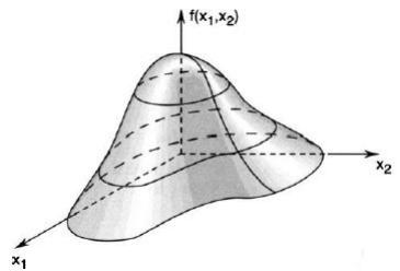
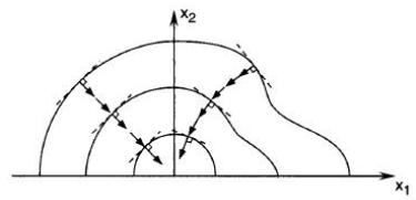
For \(f: \mathbb{R}^2 \to \mathbb{R}\) , we are usually interested in \(S\) when it is a curve. For \(f: \mathbb{R}^3 \to \mathbb{R}\) , the sets \(S\) most often considered are surfaces.

Example 5.2 Consider the following real-valued function on \(\mathbb{R}^2\) :

\[ f (\boldsymbol {x}) = 100(x _ {2} - x _ {1} ^ {2}) ^ {2} + (1 - x _ {1}) ^ {2}, \quad \boldsymbol {x} = [ x _ {1}, x _ {2} ] ^ {\top}. \]

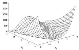
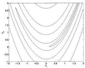
The function above is called Rosenbrock's function. A plot of the function f is shown in Figure 5.2. The level sets of f at levels 0.7, 7, 70, 200, and 700 are depicted in Figure 5.3. The figures below show the surface and its curved level sets.

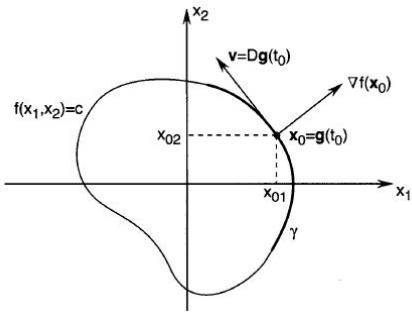
To say that a point \(x_{0}\) is on the level set S at level c means that \(f(\boldsymbol{x}_{0}) = c\) . Now suppose that there is a curve \(\gamma\) lying in S and parameterized by a continuously differentiable function \(g : R \to R^{n}\) . Suppose also that \(g(t_{0}) = x_{0}\) and \(D\boldsymbol{g}(t_{0}) = \boldsymbol{v} \neq \boldsymbol{0}\) , so that v is a tangent vector to \(\gamma\) at \(x_{0}\) (see Figure 5.4). Applying the chain rule to the function \(h(t) = f(\boldsymbol{g}(t))\) at \(t_{0}\) gives

\[ h ^ {\prime} (t _ {0}) = D f (\boldsymbol {g} (t _ {0})) D \boldsymbol {g} (t _ {0}) = D f (\boldsymbol {x} _ {0}) \boldsymbol {v}. \]

5.6 Taylor Series

演示：https://www.geogebra.org/m/rfdkjwpx

Theorem 5.8 Taylor's Theorem. Assume that a function \(f: \mathbb{R} \to \mathbb{R}\) is \(m\) times continuously differentiable (i.e., \(f \in C^m\) ) on an interval \([a, b]\) . Denote \(h = b - a\) . Then,

\[ f (b) = f (a) + \frac {h}{1 !} f ^ {(1)} (a) + \frac {h ^ {2}}{2 !} f ^ {(2)} (a) + \dots + \frac {h ^ {m - 1}}{(m - 1) !} f ^ {(m - 1)} (a) + R _ {m}, \]

(called Taylor's formula) where \(f^{(i)}\) is the \(i\) th derivative of \(f\) , and

\[ R _ {m} = \frac {h ^ {m} (1 - \theta) ^ {m - 1}}{(m - 1) !} f ^ {(m)} (a + \theta h) = \frac {h ^ {m}}{m !} f ^ {(m)} (a + \theta^ {\prime} h), \]

with \(\theta, \theta' \in (0,1)\) .

Theorem 5.9 If a function \(\pmb{f} : \mathbb{R}^n \to \mathbb{R}^m\) is differentiable on an open set \(\Omega \subset \mathbb{R}^n\) , then for any pair of points \(\pmb{x}, \pmb{y} \in \Omega\) , there exists a matrix \(M\) such that

\[ \boldsymbol {f} (\boldsymbol {x}) - \boldsymbol {f} (\boldsymbol {y}) = M (\boldsymbol {x} - \boldsymbol {y}). \]

The mean value theorem follows from Taylor's theorem (for the case where m = 1) applied to each component of f. It is easy to see that M is a matrix whose rows are the rows of Df evaluated at points that lie on the line segment joining x and y (these points may differ from row to row).

优化：Topic 1: Introduction

★ Problem

\(\min_{\boldsymbol{x}\in\Omega}f(\boldsymbol{x})\)

- \(f\) : objective function

- \(\Omega \subset \mathbb{R}^{n}\) : feasible set / constraint set

\(\max f(\boldsymbol{x})\) can be changed to \(\min -f(\boldsymbol{x})\)

1. Modeling: Practical problems → Optimization problems

2. Algorithms: Methods to solve

3. Software: Implement

Topic 1: Introduction

★ Types of Optimization Problems

- Constrained vs. Non-Constrained \(x \in \Omega\) \(x \in \mathbb{R}^{n}\) , i.e., \(x\) is free

- Convex vs. Non-convex both \(f\) and \(\Omega\) are convex

- Smooth vs. Non-Smooth \(\nabla f\) \(\partial f\) - 1-d \(R^{1}\) vs. n-d \(R^{n}\)

- illustration - motivation Harder due to infinite directions - understanding

★ Examples

1. \(\min_{x\in[0,5]}f(x)\) , \(f(x)=x^{3}-6x^{2}+9x+1\)

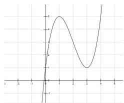
This is a 1-d smooth, non-convex, and constrained optimization sol. (only outline, not detailed solution)

critical pts: \(f'(x) = 0\) , x = 1 or x = 3

min or max ? \(f''(1) < 0\) local max, \(f''(3) > 0\) local min

Topic 1: Introduction ★ Examples Question: how about the case \(f''(x) = 0\)? Can we conclude the answer is \(x = 3\)? No! This is a constrained opt. problem. Check 1. \(x = 3 \in \Omega = [0,5]\), 2. compare with values on boundary: \(f(0), f(5)\) The final answer is \(\min_{x \in [0,5]} f(x) = 1\), and is achieved at \(x = 0, 3\). Question: Change the constraint \(\min_x f(x)\) s.t. \(x \in [-1,1]\)

Topic 1: Introduction

★ Examples

2.

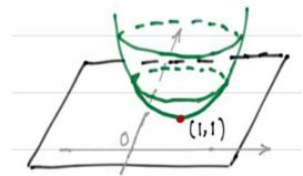
Critical pts:

\[ \begin{array}{c} f (x, y) = (x - 1) ^ {2} + (y - 1) ^ {2} \\ \min _ {(x, y) \in \mathbb {R} ^ {2}} f (x, y) \end{array} \]

\[ \left\{ \begin{array}{l l} \frac {\partial f}{\partial x} (x, y) = 0, & 2 (x - 1) = 0 \quad \Rightarrow \quad x = 1 \\ \frac {\partial f}{\partial y} (x, y) = 0, & 2 (y - 1) = 0 \quad \Rightarrow \quad y = 1 \end{array} \right. \]

★ Examples

Second order conditions.

▶ 1-d: \(f''(x) > 0\)

▶ 2-d: Hessian matrix

\[ \nabla^ {2} f = \left( \begin{array}{c c} \frac {\partial^ {2} f}{\partial x ^ {2}} & \frac {\partial^ {2} f}{\partial y \partial x} \\ \frac {\partial^ {2} f}{\partial x \partial y} & \frac {\partial^ {2} f}{\partial y ^ {2}} \end{array} \right), \text { formally } \nabla^ {2} f \succ 0 \]

For a symmetric matrix \(A = \begin{pmatrix} a_{11} & a_{12} \\ a_{21} & a_{22} \end{pmatrix}\) ,

\[ A \succ 0 \text { if } (u, v) A \binom{u}{v} > 0 \forall (u, v) \in \mathbb {R} ^ {2}, \]

i.e., \(\alpha_{11}u^{2} + 2a_{12}uv + a_{22}v^{2} > 0,\quad \forall u,v\)

特殊值: Set v = 0, u = 1 → \(a_{11} > 0\)

\[ \text { Set } u = 0, v = 1 \quad \rightarrow \quad a _ {2 2} > 0 \]

\[ \det (A) = a _ {1 1} a _ {2 2} - a _ {1 2} ^ {2} > 0 \]

Topic 1: Introduction

\(2 \times 2\) symmetric \(A \succ 0\) if \(a_{11}\) and \(\det(A) > 0\)

A can be better viewed as \(A=Q^{\top}\Lambda Q\) , where \(\Lambda = \begin{pmatrix} \lambda_{1} & 0 \\ 0 & \lambda_{2} \end{pmatrix}\) and Q consists of corresponding eigenvectors, and \(Q^{T}Q = I\)

\[ A \succ 0 \Leftrightarrow \lambda_ {1} > 0, \lambda_ {2} > 0 \]

\[ A \not\succ 0 \left\{ \begin{array}{l} \lambda_ {1} \leq 0, \lambda_ {2} \leq 0 \\ \lambda_ {1} \lambda_ {2} \leq 0 (+, -) \quad \text { saddle pt } \end{array} \right. \]

Notation. \(f:\mathbb{R}^n\to \mathbb{R}\quad \pmb {x}\in \mathbb{R}^n,\quad \pmb {x} = (x_1,x_2,\dots,x_n)\)

\[ D f \triangleq (\frac {\partial f}{\partial x _ {1}}, \frac {\partial f}{\partial x _ {2}},..., \frac {\partial f}{\partial x _ {n}}), \quad \nabla f = (D f) ^ {T} = \left( \begin{array}{c} \frac {\partial f}{\partial x _ {1}} \\ ... \\ \frac {\partial f}{\partial x _ {n}} \end{array} \right) \]

特例: 1-d, \(f'(x)\) is the slope of the tangent line \(\frac{\partial f}{\partial x_{n}}\) at x

\[ \vec {n} = (- f ^ {\prime} (x), 1) \]

\[ (x, y) \rightarrow (x, y, f (x, y)) \]

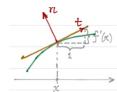
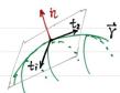
a parametrigation

\[ \vec {t} = (1, f ^ {\prime} (x)) \]

\[ \vec {t} _ {1} = \frac {\partial \vec {Y}}{\partial x} = (1, 0, \partial_ {x} f) \]

\[ \vec {t} _ {2} = \frac {\partial \vec {r}}{\partial y} = (0, 1, \partial_ {y} f) \]

\[ \vec {n} = \vec {t} _ {1} \times \vec {t} _ {2} = (- \partial_ {x} f, - \partial_ {y} f, 1) \]

\(H = \nabla^{2}f = (\frac{\partial^{2}f}{\partial x_{i}\partial x_{j}})\) . As \(\frac{\partial^2f}{\partial x_i\partial x_j} = \frac{\partial^2f}{\partial x_j\partial x_i}\) , \(\nabla^2\) is symmetric

★ Examples

1. \(\min_{x,y} f(x,y)\) s.t. \(x + y = 3\)

\[ f (x, y) = (x - 1) ^ {2} + (y - 1) ^ {2}, \quad \Omega = \{(x, y) \in \mathbb {R} ^ {2} | x + y = 3 \} \]

This is a 2-d smooth, convex and constrained optimization.

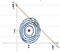
Level set \(S_{c} = \{\pmb {x}:f(\pmb {x}) = c\}\)

Level set \(S_{c}\) is a curve in \(R^{2}\)

Graph of \(f\) \((\pmb {x},f(\pmb {x}))\in \mathbb{R}^3\) is a surface in \(\mathbb{R}^3\)

Non-constrained minimum is at \((1,1)\) red pt \(\nabla f(1,1)=0\)

With an equality constraint, the minimum is changed to brown where \(\nabla f \neq 0\)

★ Examples

For this problem, we can eliminate y to get a 1-d non-constraint smooth and convex opt problem.

\[ y = 3 - x \quad \tilde {f} (x) \triangleq f (x, 3 - x) = (x - 1) ^ {2} + (x - 2) ^ {2} \]

\[ \tilde {f} ^ {\prime} (x) = 0, \mathrm{so} x = \frac {3}{2}, y = \frac {3}{2} \tilde {f} ^ {\prime \prime} (x) = 4 > 0 \forall x \]

\(x = \frac{3}{2}\) is a local minimum, and as \(\tilde{f}\) is convex, it is a global min. So \(\min f(x,y)\) s.t. \(x+y=3\) is \(\frac{1}{2}\) , and the minimum pt \((\frac{3}{2},\frac{3}{2})\)

Fact: for a convex function, a local minimum is also a global one (to be proved soon)

Topic 1: Introduction

level sets and gradient \(S_c = \{x | f(x) = c\}\). This is a smooth curve for most \(c\). How to represent/describe a curve \(f(x) = c\)? Parametrization. \(g: \mathbb{R} \to \mathbb{R}^n g(t) = (x(t), y(t))\) in \(\mathbb{R}^2\) \(h: \mathbb{R} \to \mathbb{R} h(t) \triangleq f(g(t))\) \(h(t) = c\) by definition. So \(h'(t) = 0\) By chain rule, \(h'(t) = \nabla f(g(t)) \cdot g'(t)\). So for a pt \(x_0 \in S_c\), we have \(\nabla f(x_0) \cdot v = 0\) where \(v\) is a tangent vector of \(S_c\) at \(x_0\). Theorem. \(\nabla f(x_0) \perp v\), \(\forall v\) tangent vector at \(x_0\) of the level set \(S_c\) for \(c = f(x_0)\) \(\nabla f(x)\) is the direction of maximum rate of increase of \(f\) at \(x\) -\(\nabla f(x)\) is the direction of maximum rate of decrease of \(f\) at \(x\) -\(\nabla f(x)\): steepest descent direction

level sets and gradient \(S_c = \{x | f(x) = c\}\). This is a smooth curve for most \(c\). How to represent/describe a curve \(f(x) = c\)? Parametrization. \(g: \mathbb{R} \to \mathbb{R}^n g(t) = (x(t), y(t))\) in \(\mathbb{R}^2\) \(h: \mathbb{R} \to \mathbb{R} h(t) \triangleq f(g(t))\) \(h(t) = c\) by definition. So \(h'(t) = 0\) By chain rule, \(h'(t) = \nabla f(g(t)) \cdot g'(t)\). So for a pt \(x_0 \in S_c\), we have \(\nabla f(x_0) \cdot v = 0\) where \(v\) is a tangent vector of \(S_c\) at \(x_0\). Theorem. \(\nabla f(x_0) \perp v\), \(\forall v\) tangent vector at \(x_0\) of the level set \(S_c\) for \(c = f(x_0)\) \(\nabla f(x)\) is the direction of maximum rate of increase of \(f\) at \(x\) \(-\nabla f(x)\) is the direction of maximum rate of decrease of \(f\) at \(x\) \(-\nabla f(x)\): steepest descent direction

★ Examples

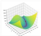
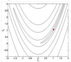
1. Rosenbrock function \(f(x_{1},x_{2}) = 100(x_{2} - x_{1}^{2})^{2} + (1 - x_{1})^{2}\)

\[ \min _ {\boldsymbol {x} \in \mathbb {R} ^ {2}} f \]

non-constrained, smooth, but non-convex

\(\nabla f(\boldsymbol {x}) = \binom{-400x_{1}(x_{2} - x_{1}^{2}) - 2(1 - x_{1})}{200(x_{2} - x_{1}^{2})}\) , critical point (1,1)

\[ H(\boldsymbol{x})=\nabla^2 f(\boldsymbol{x})=\begin{pmatrix}1200x_1^2-400x_2+2 & -400x_1 \\ -400x_1 & 200\end{pmatrix} \]

\(H(1,1) = \left( \begin{array}{cc}802 & -400\\ -400 & 200 \end{array} \right),\) so \((1,1)\) is a local minimum.

(1, 1) is also a global minimum. It is inside a long, narrow, parabolic shaped flab valley.

6.1 习题

\[ \begin{array}{l l} \text { minimize } & f (\boldsymbol {x}) \\ \text { subject to } & \boldsymbol {x} \in \Omega , \end{array} \]

where \(f \in C^{2}\) . For each of the following specifications for \(\Omega\) , \(x^{*}\) , and f, determine if the given point \(x^{*}\) is: (i) definitely a local minimizer; (ii) definitely not a local minimizer; or (iii) possibly a local minimizer.

b. \(f: \mathbb{R}^2 \to \mathbb{R}\) , \(\Omega = \{\pmb{x} = [x_1, x_2]^{\top}: x_1 \geq 1, x_2 \geq 2\}\) , \(\pmb{x}^* = [1, 2]^{\top}\) , and gradient \(\nabla f(\pmb{x}^*) = [1, 0]^{\top}\) .

习题

6.1 Consider the problem

\[ \begin{array}{l l} \text { minimize } & f (\boldsymbol {x}) \\ \text { subject to } & \boldsymbol {x} \in \Omega , \end{array} \]

where \(f \in C^{2}\) . For each of the following specifications for \(\Omega\) , \(x^{*}\) , and f, determine if the given point \(x^{*}\) is: (i) definitely a local minimizer; (ii) definitely not a local minimizer; or (iii) possibly a local minimizer.

c. \(f: \mathbb{R}^2 \to \mathbb{R}\) , \(\Omega = \{\pmb{x} = [x_1, x_2]^{\top}: x_1 \geq 0, x_2 \geq 0\}\) , \(\pmb{x}^* = [1, 2]^{\top}\) , gradient \(\nabla f(\pmb{x}^*) = [0, 0]^{\top}\) , and Hessian \(\pmb{F}(\pmb{x}^*) = \pmb{I}\) (identity matrix).

d. \(f:\mathbb{R}^2\to \mathbb{R},\Omega = \{\pmb {x} = [x_1,x_2]^{\top}:x_1\geq 1,x_2\geq 2\} ,\pmb{x}^{*} = [1,2]^{\top}\) gradient \(\nabla f(\pmb{x}^{*}) = [1,0]^{\top}\) ,and Hessian

\[ \boldsymbol {F} (\boldsymbol {x} ^ {*}) = \left[ \begin{array}{c c} 1 & 0 \\ 0 & - 1 \end{array} \right]. \]

知识点、重点、难点

知识点

- 优化问题的一般形式：

\[ \min _ {\boldsymbol {x} \in \Omega} f (\boldsymbol {x}) \]

其中 \(f(x)\) 为目标函数， \(\Omega\) 为约束集合。

- 优化问题的主要分类：有约束 / 无约束、凸 / 非凸、光滑 / 非光滑。

- 局部最小点与全局最小点的概念。

- 梯度（Gradient）与 Hessian 矩阵在多维函数中的几何意义。

知识点、重点、难点

重点

优化问题的核心在于通过一阶条件 \(\nabla f(x)=0\) 寻找候选极值点，并利用二阶条件（Hessian 的正定性）判断其为极小点；凸函数中局部最小即为全局最小，而含约束问题则常可通过变量消元化为无约束形式。

难点

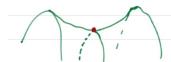
- 区分局部最小点、鞍点与约束最小点。

- 约束优化中如何判断最优解是否在边界上。

一句话总结：

本节核心在于理解优化问题的建模、分类与基本求解原则，掌握梯度和 Hessian 在判断极值中的作用，为后续最优条件的学习奠定基础。