2026-10-11 · 最优性与搜索

高级工程数学

2026-10-11

沈超敏

计算机科学与技术学院

cmshen@cs.ecnu.edu.cn

文附楼 105

今天内容

1. 上次内容（Ch. 5、Ch. 6 (Topic 1. Introduction)）的复习拓展
2. Topic 2: Optimality Conditions
3. Ch. 7
4. Gradient Methods
5. Newton’s Methods

上次: Elements of Calculus 5.1 Sequences and Limits 5.2 Differentiability 5.3 The Derivative Matrix 5.4 Differentiation Rules 5.5 Level Sets and Gradients 5.6 Taylor Series

Topic 1 回顾

知识点

优化问题的一般形式：

\[ \min _ {\boldsymbol {x} \in \Omega} f (\boldsymbol {x}) \]

其中 f(x) 为目标函数，Ω 为约束集合。

优化问题的主要分类：有约束 / 无约束、凸 / 非凸、光滑 / 非光滑。

局部最小点与全局最小点的概念。

梯度（Gradient）与 Hessian 矩阵在多维函数中的几何意义。

Topic 1 的知识点、重点、难点

重点

优化问题的核心在于通过一阶条件 ∇f(x) = 0 寻找候选极值点，并利用二阶条件（Hessian 的正定性）判断其为极小点；凸函数中局部最小即为全局最小，而含约束问题则常可通过变量消元化为无约束形式。

Topic 1 的难点

区分局部最小点、鞍点与约束最小点。

约束优化中如何判断最优解是否在边界上。

一句话总结：

本节核心在于理解优化问题的建模、分类与基本求解原则，掌握梯度和 Hessian 在判断极值中的作用，为后续最优条件的学习奠定基础。

上次：习题

6.1 习题

\[ \begin{array}{l l} \text { minimize } & f (\boldsymbol {x}) \\ \text { subject to } & \boldsymbol {x} \in \Omega , \end{array} \]

where \(f \in { \mathcal { C } } ^ { 2 }\) . For each of the following specifications for \(\Omega , { \pmb x } ^ { * }\) , and \(f ,\) , determine if the given point \({ \pmb x } ^ { * }\) is: (i) definitely a local minimizer; (ii) definitely not a local minimizer; or (iii) possibly a local minimizer.

b. \(\begin{array} { r l } & { f : \mathbb { R } ^ { 2 } \to \mathbb { R } , \Omega = \{ { \pmb x } = [ { \pmb x } _ { 1 } , { \pmb x } _ { 2 } ] ^ { \top } : x _ { 1 } \geq 1 , { \pmb x } _ { 2 } \geq 2 \} , { \pmb x } ^ { * } = [ 1 , 2 ] ^ { \top } } \\ & { \nabla f ( { \pmb x } ^ { * } ) = [ 1 , 0 ] ^ { \top } . } \end{array}\).

答案：Possibly a local minimizer

c. \(f : \mathbb { R } ^ { 2 } \to \mathbb { R } , \Omega = \lbrace x = [ x _ { 1 } , x _ { 2 } ] ^ { \top } : x _ { 1 } \geq 0 , x _ { 2 } \geq 0 \rbrace , x ^ { * } = [ 1 , 2 ] ^ { \top }\) , gradient \(\nabla f ( \pmb { x } ^ { * } ) = [ 0 , 0 ] ^ { \top }\) , and Hessian \(\pmb { F } ( \pmb { x } ^ { * } ) = \pmb { I }\) (identity matrix).

d. \(f : \mathbb{R}^{2}\to\mathbb{R}\), \(\Omega=\{\pmb{x}=[x_1,x_2]^\top:x_1\geq1,x_2\geq2\}\), \(\pmb{x}^*=[1,2]^\top\), gradient \(\nabla f ( { \pmb x } ^ { * } ) = [ 1 , 0 ] ^ { \top }\) , and Hessian

\[ \boldsymbol {F} (\boldsymbol {x} ^ {*}) = \left[ \begin{array}{c c} 1 & 0 \\ 0 & - 1 \end{array} \right]. \]

C 是, D 不是

Topic 2: Optimality Conditions

Three acronyms:

FONC (First Order Necessary Condition)

SONC (Second Order Necessary Condition)

SOSC (Second Order Sufficient Condition)

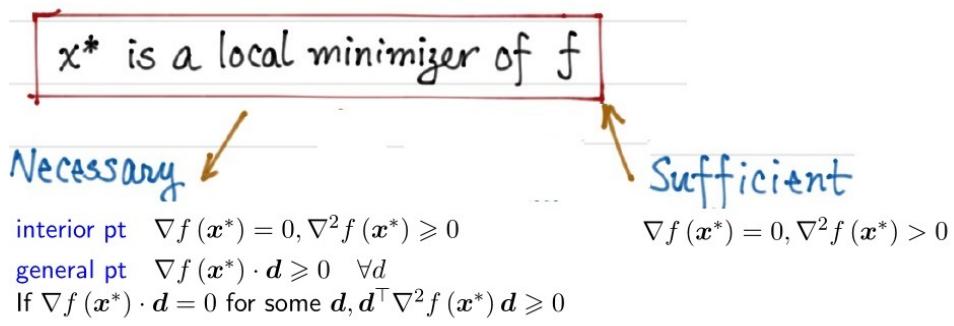
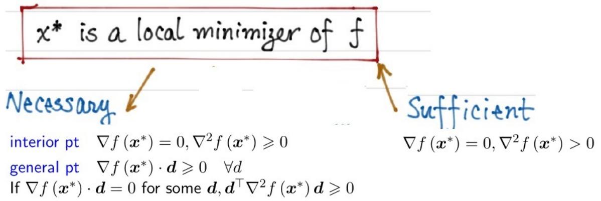
interior pt ∇f (x*) = 0, ∇2 f (x*) ≥ 0

general pt ∇f (x*) · d ≥0 ∀d

Topic 2: Condition

⋆ Conditions for Local Minimizers

Global minimizer \(\pmb { x } ^ { \ast } : f ( \pmb { x } ) \geqslant f \left( \pmb { x } ^ { \ast } \right) \quad \forall \pmb { x } \in \Omega \backslash \left\{ \pmb { x } ^ { \ast } \right\}\)

Strict global minimizer \(\pmb { x } ^ { \ast } : f ( \pmb { x } ) > f \left( \pmb { x } ^ { \ast } \right) \quad \forall \pmb { x } \in \Omega \backslash \left\{ \pmb { x } ^ { \ast } \right\}\)

Mathematically, “near” can be characterized as \(\| { \pmb x } - { \pmb x } ^ { * } \| < \varepsilon\)

● \(\scriptstyle { \pmb { x } } ^ { * }\) is a local minimizer if ∃ε > 0, s.t.

\[ f (\boldsymbol {x}) \geqslant f \left(\boldsymbol {x} ^ {*}\right) \quad \forall \boldsymbol {x} \in \Omega \backslash \left\{\boldsymbol {x} ^ {*} \right\} \& \| \boldsymbol {x} - \boldsymbol {x} ^ {*} \| < \varepsilon \]

Topic 2: Condition

⋆ First Order Necessary Condition

Theorem. \(\mathbf { \boldsymbol { x } } ^ { * }\) is a local minimizer of f over Ω. Then for any feasible direction d at \(\mathbf { \boldsymbol { x } } ^ { * }\) , we have

\[ \nabla f \left(\boldsymbol {x} ^ {*}\right) \cdot \boldsymbol {d} \geqslant 0 \]

Explanation. 1 feasible direction d at a point \(\pmb { x } \in \Omega\) is a direction so that: starting from x and moving towards d remains in Ω.

Math language: ∃α > 0 s.t. \(\pmb { x } + \alpha \pmb { d } \in \Omega , \forall \alpha \in [ 0 , \alpha _ { 0 } ]\)

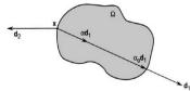
2 \(\nabla f \left( \mathbf { x } ^ { * } \right) \cdot d\) : inner product of two vectors.

Also write as \(\begin{array} { r l r l } { d ^ { \top } \nabla f \left( { \pmb x } ^ { * } \right) } & { { } \mathrm { o r } } & { \left( \nabla f \left( { \pmb x } ^ { * } \right) , { \pmb d } \right) , } & { \left. \nabla f \left( { \pmb x } ^ { * } \right) , { \pmb d } \right. } \end{array}\)

\({ \frac { \partial f } { \partial d } } \triangleq \nabla f\) · d is the directional derivative when \(\| \pmb { d } \| = 1\)

3 Define \(\phi ( \alpha ) = f \left( \boldsymbol { x } ^ { * } + \alpha d \right)\) for \(\alpha \in [ 0 , \alpha _ { 0 } ]\) , then

\[ \phi^ {\prime} (0) = \left\{ \begin{array}{l l} \lim _ {\alpha \to 0 ^ {+}} \frac {\phi (\alpha) - \phi (0)}{\alpha} = \lim _ {\alpha \to 0 ^ {+}} \frac {f (\boldsymbol {x} ^ {*} + \alpha \boldsymbol {d}) - f (\boldsymbol {x} ^ {*})}{\alpha} & \text {Def} \\ \nabla f \left(\boldsymbol {x} ^ {*}\right) \cdot \boldsymbol {d} & \text {Chain rule} \end{array} \right. \]

Topic 2: Condition

Proof. Let d be any feasible direction at \(\scriptstyle { \pmb { x } } ^ { * }\)

Define \(\phi ( \alpha ) = f \left( \boldsymbol { x } ^ { * } + \alpha \boldsymbol { d } \right)\) ，then

\[ \begin{array}{r c l} f \left(\boldsymbol {x} ^ {*} + \alpha \boldsymbol {d}\right) - f \left(\boldsymbol {x} ^ {*}\right) & = & \phi (\alpha) - \phi (0) = \phi^ {\prime} (0) \alpha + o (\alpha) \\ & = & \langle \nabla f \left(\boldsymbol {x} ^ {*}\right) \cdot \boldsymbol {d} \rangle \alpha + o (\alpha) \end{array} \]

If \(\scriptstyle { \pmb { x } } ^ { * }\) is a local minimizer,

\[ \left(\text { i.e., } \exists \varepsilon , \text { s.t. } f (\boldsymbol {x}) \geqslant f \left(\boldsymbol {x} ^ {*}\right), \forall \boldsymbol {x} \in \Omega \backslash \left\{\boldsymbol {x} ^ {*} \right\} \& \| \boldsymbol {x} - \boldsymbol {x} ^ {*} \| < \varepsilon\right) \]

for sufficiently small \(\alpha\) (e.g., when \(\|\alpha\pmb{d}\|<\varepsilon\)), we have \(f(\pmb{x}^*+\alpha\pmb{d})-f(\pmb{x}^*)\geq0\). Then

\[ \phi^ {\prime} (0) = \nabla f \left(\boldsymbol {x} ^ {*}\right) \cdot \boldsymbol {d} \geqslant 0 \]

FONC Two possibilities for a given feasible direction d.

\(\nabla f(x^*)\cdot d>0\): \(f(x^*+\alpha d)>f(x^*)\) for all sufficiently small \(\alpha>0\).

\(\nabla f(x^*)\cdot d=0\): check the second-order derivative.

⋆ Second Order Necessary Condition

Theorem If \(\mathbf { \boldsymbol { x } } ^ { * }\) is a local minimizer of \(f\) over \(\Omega ,\) and there exists a feasible direction d at \(\scriptstyle { \pmb { x } } ^ { * }\) s.t. \(\nabla f \left( \pmb { x } ^ { * } \right) \cdot \pmb { d } = 0\) , then

\[ \boldsymbol {d} ^ {\top} \nabla^ {2} f (\boldsymbol {x} ^ {*}) \boldsymbol {d} \geqslant 0 \]

Proof Consider \(\phi ( \alpha ) = f \left( \boldsymbol { x } ^ { * } + \alpha d \right)\) and its Taylor series at \(\alpha = 0\)

\[ \phi (\alpha) = \phi (0) + \phi^ {\prime} (0) \alpha + \frac {1}{2} \phi^ {\prime \prime} (0) \alpha^ {2} + o \left(\alpha^ {2}\right). \]

\[ \text { as } \phi^ {\prime} (0) = \nabla f (\boldsymbol {x} ^ {*}) \cdot \boldsymbol {d} = 0 \]

So we have \(\begin{array} { r } { \phi ( \alpha ) - \phi ( 0 ) = \frac { 1 } { 2 } \phi ^ { \prime \prime } ( 0 ) \alpha ^ { 2 } + o \left( \alpha ^ { 2 } \right) } \end{array}\) . Written in terms f is \(f \left( \pmb { x } ^ { * } + \alpha \pmb { d } \right) - f \left( \pmb { x } ^ { * } \right) =\) \(\begin{array} { r } { \frac { \alpha ^ { 2 } } { 2 } \pmb { d } ^ { \top } \nabla ^ { 2 } f \left( x ^ { * } \right) \pmb { d } + o \left( \alpha ^ { 2 } \right) } \end{array}\)

If \(\pmb { d } ^ { \top } \nabla ^ { 2 } f \left( \pmb { x } ^ { * } \right) \pmb { d } < 0\) , then for sufficiently small \(\alpha\) (how small?)

which contradicts that \(x ^ { * }\) is a local minimizer.

so, \(\pmb { d } ^ { \top } \nabla ^ { 2 } f \left( \pmb { x } ^ { * } \right) \pmb { d } \geq 0 .\)

Topic 2: Condition

Corollary \(\mathbf { x } ^ { \ast }\) is an interior local minimizer of f. Then

FONC \(\nabla f \left( \pmb { x } ^ { * } \right) = 0\)

SONC: \(d^{\top}\nabla^{2}f(\pmb{x}^{*})d\geq 0\) for all \(d\in\mathbb{R}^{n}\).

Examples. 6.3 (p.86), 6.5 (p.89)

Necessary conditions are not sufficient

\[ f (x) = x ^ {3}, f ^ {\prime} (x) = 3 x ^ {2}, f ^ {\prime \prime} (x) = 6 x \]

\[ f (\pmb {x}) = x _ {1} ^ {2} - x _ {2} ^ {2} \]

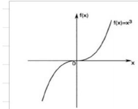
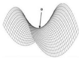
0 is a saddle point \(\nabla f ( \mathbf { 0 } ) = \mathbf { 0 }\) but neither a local minimizer nor maximizer By SONC, 0 is not a local minimizer!

⋆ Second Order Sufficient Condition

Th 6.3 (SOSC) \(f \in C ^ { 2 } ( \Omega ) , x ^ { * } \in \Omega\) is an interior point.

Suppose that (1) \(\nabla f \left( { { \pmb x } ^ { * } } \right) = { \bf 0 } ; \left( 2 \right) \nabla ^ { 2 } f \left( { { \pmb x } ^ { * } } \right) \succ 0 .\)

Then \(\mathbf { \boldsymbol { x } } ^ { * }\) is a strict local minimizer of \(f .\)

Pf. \(\nabla ^ { 2 } f \left( x ^ { * } \right) \succ 0 \Leftrightarrow \lambda _ { \operatorname* { m i n } } \left( \nabla ^ { 2 } f \left( x ^ { * } \right) \right) > 0\)

(Diagonalize \(\nabla^2f(\mathbf{x}^*)=Q^\top\Lambda Q\).)

For a feasible direction \(d\neq 0\), define \(\phi(\alpha)=f(\boldsymbol{x}^*+\alpha\boldsymbol{d})\).

\[ \begin{array}{r l} & f (\boldsymbol {x} ^ {*} + \alpha \boldsymbol {d}) - f (\boldsymbol {x} ^ {*}) = \phi (\alpha) - \phi (0) = \frac {1}{2} \phi^ {\prime \prime} (0) \alpha^ {2} + o (\alpha^ {2}) \\ & \qquad = \frac {1}{2} \boldsymbol {d} ^ {\top} \nabla^ {2} f (\boldsymbol {x} ^ {*}) \boldsymbol {d} \alpha^ {2} + o (\alpha^ {2}) \\ & \qquad \geqslant \frac {1}{2} \lambda_ {\min} \| d \| ^ {2} \alpha^ {2} + o (\alpha^ {2}) > 0 \end{array} \]

if α is sufficiently small.

习题

6.1 Consider the problem

\[ \begin{array}{l l} \text { minimize } & f (\boldsymbol {x}) \\ \text { subject to } & \boldsymbol {x} \in \Omega , \end{array} \]

where \(f \in { \mathcal { C } } ^ { 2 }\) . For each of the following specifications for \(\Omega , { \pmb x } ^ { * }\) , and \(f ,\) , determine if the given point \({ \pmb x } ^ { * }\) is: (i) definitely a local minimizer; (ii) definitely not a local minimizer; or (iii) possibly a local minimizer.

a. \(\begin{array} { r l } & { f : \mathbb { R } ^ { 2 } \to \mathbb { R } , \Omega = \{ \mathbf { x } = [ x _ { 1 } , x _ { 2 } ] ^ { \top } : x _ { 1 } \geq 1 \} , \mathbf{x} ^ { * } = [ 1 , 2 ] ^ { \top } } \\ & { \nabla f ( \mathbf { x } ^ { * } ) = [ 1 , 1 ] ^ { \top } . } \end{array}\) , and gradient

一定不是

3. 几何直观

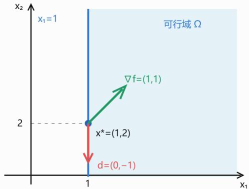
• 绿色箭头：梯度方向，函数值上升最快

• 红色箭头：可行的下降方向，函数值减小。

• 蓝色直线：约束边界 \(x _ { 1 } = 1 ,\)

Ch 7. One-Dimensional Search Methods

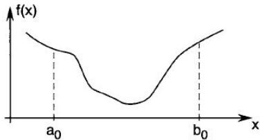
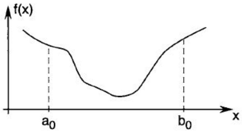
7.1 Introduction

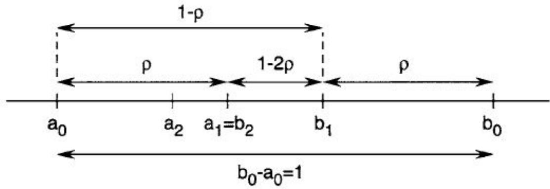
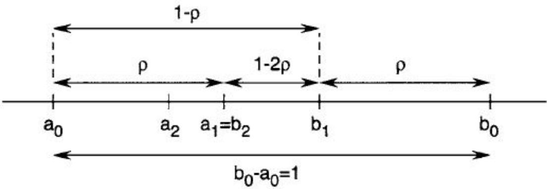
7.2 Golden Section Search

7.3 Fibonacci Method

7.4 Bisection Method

7.5 Newton’s Method

7.6 Secant Method

7.7 Bracketing

7.8 Line Search in Multidimensional Optimization

§2 单因素

我们知道，钢要用某种化学元素来加强其强度，太少不好，太多也不好，例如，碳太多了成为生铁，碳太少了成为熟铁，都不成钢材，每吨要加多少碳才能达到强度最高？假定从理论上算出)每吨在1000克到2000克之间，普通的方法是加1001克，1002克，……，做下去，做了一千次以后，才能发现最好的选择，这种方法称为均分法，做一千次实验既浪费时又浪费原材料，为了迅速找出最优方案，我们建议以下的“折迭纸条法”

请牢记一个数0.618

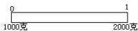
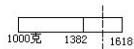
用一个有刻度的纸条表达1000\~2000克，在这纸条长度的0.618的地方划一条线，在这条线所指示的刻度做一次实验，也就是按1618克做一次实验

然后把纸条对中迭起，前一线落在另一层上的地方，再划一条线，这条线在1382克处，再按1382克做一次实验

两次实验进行比较，如果1382克的好一些，我们在1618处把纸条的右边一段剪掉，得

Ch 7. One-Dimensional Search Methods

7.3 Fibonacci Method

Topic 3: Ch 8. Gradient Methods

\(\nabla f ( x )\) is the direction of maximum rate of increase of f at x.

\(- \nabla f ( x )\) is the direction of maximum rate of decrease of f at x.

Lemma (Cauchy–Schwarz inequality). For \(\boldsymbol{a},\boldsymbol{b}\in\mathbb{R}^n\),

\[ \boldsymbol {a} \cdot \boldsymbol {b} = (\boldsymbol {a}, \boldsymbol {b}) = \sum_ {i = 1} ^ {n} a _ {i} b _ {i} \leqslant \left(\sum_ {i = 1} ^ {n} a _ {i} ^ {2}\right) ^ {\frac {1}{2}} \left(\sum_ {i = 1} ^ {n} b _ {i} ^ {2}\right) ^ {\frac {1}{2}} = \| \boldsymbol {a} \| \cdot \| \boldsymbol {b} \| \]

Pf: Consider

\[ \begin{array}{r l} & y (t) = \left(\sum a _ {i} ^ {2}\right) t ^ {2} + \left(2 \sum a _ {i} b _ {i}\right) t + \sum b _ {i} ^ {2} \\ & \quad = \sum_ {i = 1} ^ {n} \left(a _ {i} ^ {2} t ^ {2} + 2 a _ {i} b _ {i} t + b _ {i} ^ {2}\right) \\ & \quad = \sum (a _ {i} t + b _ {i}) ^ {2} \geqslant 0 \end{array} \]

\(y ( t ) = 0\) if \(a _ { i } t + b _ { i } = 0 ,\) , ∀i

\[ \mathrm{So} \Delta = (2 \Sigma a _ {i} b _ {i}) ^ {2} - 4 (\Sigma a _ {i} ^ {2}) (\Sigma b _ {i} ^ {2}) \leqslant 0 \]

Topic 3: Gradient Methods

Apply to \(( \nabla f , d ) \leqslant \| \nabla f \| \cdot \| d \| = \| \nabla f \| { \mathrm { ~ i f ~ } } \| d \| = 1\)

Equality holds \(\begin{array} { r } { \Leftrightarrow d = \frac { \nabla f } { \| \nabla f \| } } \end{array}\)

Therefore \(- \nabla f ( { \pmb x } )\) is the max-rate descending direction. When \(\nabla f ( { \pmb x } ) \neq { \bf 0 }\) , for α sufficiently small, \(f ( { \pmb x } - \alpha \nabla f ( { \pmb x } ) ) < f ( { \pmb x } )\)

Topic 3: Gradient Methods

Gradient Descent Algorithm:

Start from \(\mathbf { x } ^ { 0 }\) for \(k = 0 , 1 , 2 , \cdots\) till converge

\[ \boldsymbol {x} ^ {k + 1} = \boldsymbol {x} ^ {k} - \alpha_ {k} \nabla f (\boldsymbol {x} ^ {k}) \]

Ideal condition: \(\left\| \nabla f \left( { \boldsymbol { x } } ^ { k } \right) \right\| = 0\)

Practical conditions:

gradient condition \(\left\| \nabla f \left( \mathbf { x } ^ { k } \right) \right\| < \varepsilon\)

success objective condition \(\frac { \left| f \big ( x ^ { k + 1 } \big ) - f \big ( x ^ { k } \big ) \right| } { \left| f \big ( x ^ { k } \big ) \right| } < \varepsilon\)

successive point difference \(\frac { \left\| \mathbf { { x } } ^ { k + 1 } - \mathbf { { x } } ^ { k } \right\| } { \left\| \mathbf { { x } } ^ { k } \right\| } < \varepsilon\)

Replace denominator by max \(\left\{ 1 , \left| f \left( \pmb { x } ^ { k } \right) \right| \right\}\) or max \(\{ 1 , \| \pmb { x } ^ { k } \| \}\) to avoid division by tiny numbers

Topic 3: Gradient Methods Step size:

1. Exact line search. Expensive and not worth

2. Fixed estimate value.

3. Line search (Ch. 7).

具体地

1. Exact or “best” for \(\phi _ { k } ( \alpha ) = f \left( x _ { k } - \alpha \nabla f \left( x _ { k } \right) \right)\)

\[ \alpha_ {k} = \underset {\alpha \geqslant 0} {\arg \min} \phi_ {k} (\alpha) \]

This is called Steepest Descent method.

梯度下降法的性质：相邻方向垂直

\[ \alpha_ {k} = \arg \min _ {\alpha \geq 0} f (x _ {k} - \alpha \nabla f (x _ {k})). \]

令

\[ \phi (\alpha) = f (x _ {k} - \alpha \nabla f (x _ {k})). \]

由于 \(\alpha _ { k }\) 是内部极小点，所以

利用链式法则

\[ \phi^ {\prime} (\alpha_ {k}) = 0. \]

\[ \phi^ {\prime} (\alpha) = - \nabla f (x _ {k} - \alpha \nabla f (x _ {k})) ^ {T} \nabla f (x _ {k}). \]

代入 \(\alpha _ { k }\) ，得到

\[ - \nabla f (x _ {k + 1}) ^ {T} \nabla f (x _ {k}) = 0. \]

因此

\[ \boxed {\nabla f (x _ {k + 1}) ^ {T} \nabla f (x _ {k}) = 0} \]

Topic 3: Gradient Methods

1. Based on properties of f, choose a fixed value

small: converges slow

large: may diverge faster

convergence eficiency

1. Several practical line search algorithms

• Golden section • Newton’s method

• Fibonacci • Secant method

梯度下降法缺点

作业

编写一个完整的最速下降算法，

1. 定义 f(x)

2. 给出 \(\scriptstyle { \pmb { x } } ^ { * }\) 的算法

运行时，输入 f(x) 和 \(\scriptstyle { \mathbf { { \mathit { x } } } } _ { 0 }\)

输出 \(\mathbf { \boldsymbol { x } } ^ { * }\)

Consider \(\min_{x\in\mathbb{R}^{n}}f(x)\) \(\cdot n=1\) \(x_{k+1}=x_{k}-\left(f''(x_{k})\right)^{-1}f'(x_{k})\) \(\cdot n>1\) \(x_{k+1}=x_{k}-\left(\nabla^{2}f(x_{k})\right)^{-1}\nabla f(x_{k})\)

Another form ① solve \(\nabla^{2}f(x_{k})d_{k}=-\nabla f(x_{k})\) ② update \(x_{k+1}=x_{k}+d_{k}\)

Remark. Do not require \(\nabla^{2}f(x_{k})>0\) only needs non-singular (invertible). Namely, Newton's method also works for non-convex optimization problems. but may not find local min.

Topic 4: Newton’s method

Pro. 1. Converges super-fast (quadratic rate).

1. Affine invariant.

Cons. 1. Local convergence; requires \(\|x_0-x^*\|\) to be sufficiently small.

1. Computational cost: forming the Hessian costs \(O(n^2)\), and computing \((\nabla^2f)^{-1}\) costs \(O(n^3)\).

Topic 4: Newton’s method

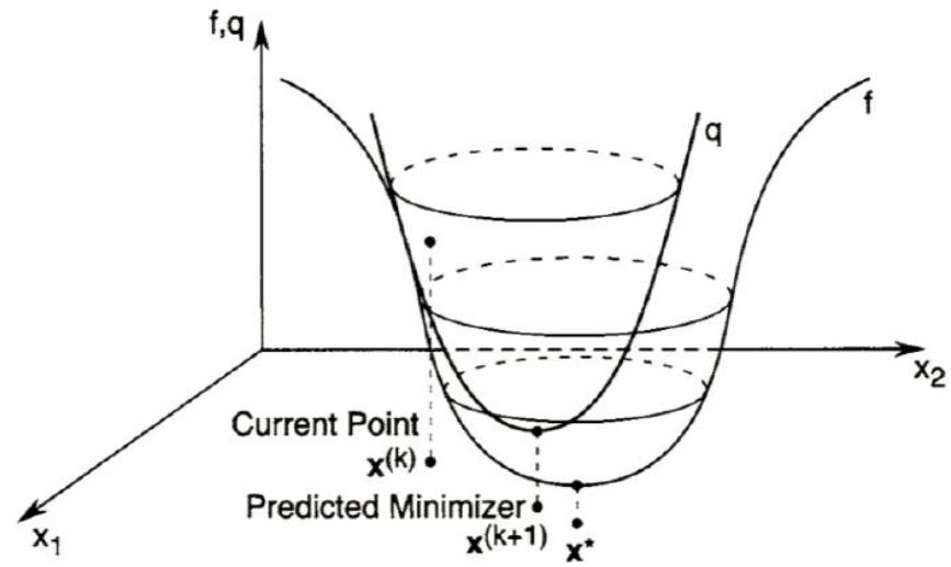
Derivation, Given current approximate xk, approximates f by its quadratic Taylor series

\[ f (x) \approx f _ {g} (x; x _ {k}) := f (x _ {k}) + (\nabla f (x _ {k}), x - x _ {k}) + \frac {1}{2} (\nabla^ {2} f (x _ {k}) (x - x _ {k}), x - x _ {k}) \]

\[ \begin{array}{l l} {\underset {x \in \mathbb {R} ^ {n}} {\min} f (x)} & {\longrightarrow \underset {x \in \mathbb {R} ^ {n}} {\min} f _ {\mathfrak {g}} (x; x _ {k}) \longrightarrow \nabla f _ {\mathfrak {g}} (x _ {k + 1}; x _ {k}) = 0.} \\ & {\quad \downarrow} \\ {\nabla f _ {\mathfrak {g}} (x; x _ {k}) = \nabla f (x _ {k}) + \nabla^ {2} f (x _ {k}) (x - x _ {k})} & {\mathrm {Newton^ {\prime} s method}} \end{array} \]

Topic 4: Newton’s method

Convergence Analysis.

Theorem. Suppose \(f\in C^3\), \(x^*\) is a critical point, i.e., \(\nabla f(x^*)=0\), and \(\nabla^2f(x^*)\) is invertible. Then for all \(x_0\) sufficiently close to \(x^*\), Newton’s method is well defined for all \(k\) and satisfies \(\|x_{k+1}-x^*\|\leq C\|x_k-x^*\|^2\) for \(k=0,1,2,\ldots\). Proof. Denote \(F(x)=\nabla^2f(x)\). Then \(\det F(x)\in C^1\). Since \(\det F(x^*)\ne0\), for sufficiently small \(\varepsilon>0\), \(\det F(x)\ne0\) whenever \(\|x-x^*\|<\varepsilon\). Thus \(F(x)\) is invertible.

Furthermore \(\| F^{-1}(x) \| \leqslant c\), \(\forall \| x - x^* \| < \varepsilon\).

Assume \(x_k\) satisfies \(\| x_k - x^* \| < \varepsilon\), then \(F^{-1}(x_k)\) exists and \(\| F^{-1}(x_k) \| \leqslant c\).

Then \(x_{k+1} - x^* = x_k - x^* - (\nabla^2 f(x_k))^{-1} \nabla f(x_k)\) \(= (\nabla^2 f(x_k))^{-1} [\nabla^2 f(x_k)(x_k - x^*) - \nabla f(x_k)]\).

We apply first order Taylor expansion to \(\nabla f(x^*)\) at \(x_k\) to get

\(\nabla f(x^*) = \nabla f(x_k) + \nabla^2 f(x_k)(x^* - x_k) + O(\| x_k - x^* \|^2)\)

Note that \(\nabla f(x^*) = 0\) and the sign change, we have

\(\nabla^2 f(x_k)(x_k - x^*) - \nabla f(x_k) = O(\| x_k - x^* \|^2)\).

Therefore \(\| x_{k+1} - x^* \| \leqslant C\|\left(\nabla^2 f(x_k)\right)^{-1} \| \| x_k - x^* \|^2\) \(\leqslant C_1 \| x_k - x^* \|^2\)

Topic 4: Newton’s method

Topic 4: Newton’s method

Choosing \(\varepsilon\) smaller if necessary so that \(C_1\varepsilon^2<\varepsilon\), we conclude that \(\|x_{k+1}-x^*\|<\varepsilon\) and \(F(x_{k+1})^{-1}\) exists with \(\|F(x_{k+1})^{-1}\|\leq C\). Thus, if \(\|x_0-x^*\|<\varepsilon\), then \(\|x_k-x^*\|<\varepsilon\) and \(\|x_{k+1}-x^*\|\leq C_1\|x_k-x^*\|^2\) for all \(k=0,1,2,\ldots\), which implies local quadratic convergence.

Modification of Newton's method.

Newton's method may not be a descent method, i.e. \(f(x_{k+1}) > f(x_k)\) is possible (e.g. \(x^*\) is a local maximum). Have to restrict to strictly convex functions.

Lemma. Assume \(\nabla^2 f(x) > 0, \forall x\). If \(\nabla f(x_k) \neq 0\), then Newton's direction \(d_k = -(\nabla^2 f(x_k))^{-1} \nabla f(x_k)\) is a descent direction in the sense that \(f(x_k+\alpha d_k)<f(x_k)\) for all sufficiently small \(\alpha>0\).

Proof. Let \(\phi(\alpha)=f(x_k+\alpha d_k)\). Then

\[\phi'(0)=\nabla f(x_k)^\top d_k=-\nabla f(x_k)^\top(\nabla^2f(x_k))^{-1}\nabla f(x_k)<0,\]

because \(\nabla^2f(x_k)\) is positive definite.

Topic 4: Newton’s method

For convex functions, use the following modification:

1. Compute \(d_k\) by solving \(\nabla^2f(x_k)d_k=-\nabla f(x_k)\).
2. Find \(\alpha_k=\arg\min_{\alpha\geq0}f(x_k+\alpha d_k)\) by line search.
3. Update \(x_{k+1}=x_k+\alpha_kd_k\).

What if \(\nabla^{2}f\) is not SPD? Note that for non-convex functions, the gradient method \(x_{k+1}=x_{k}-\alpha_{k}I\nabla f(x_{k})\) is always a descent method. This motivates the Levenberg-Marquardt modification

\[ x _ {k + 1} = x _ {k} - \alpha_ {k} (\nabla^ {2} f (x _ {k}) + \mu_ {k} I) ^ {- 1} \nabla f (x _ {k}), \]

where \(\mu_k>0\) is chosen so that \(\nabla^2f(x_k)+\mu_k I\) is positive definite, and \(\alpha_k>0\) is a step size.

It is a mixture of Newton and gradient methods:

μk=0. Newton's method.

\(\mu_k\to+\infty\). Gradient method.