2026-10-25 · KKT 与近端方法

高级工程数学

2026-10-25

沈超敏

计算机科学与技术学院

cmshen@cs.ecnu.edu.cn

文附楼 105

今天内容

复习、拓展

Lagrange 乘子法

The Karush–Kuhn–Tucker (KKT) Conditions

Proximal Gradient 方法

Subgradient 方法

上次：Lagrange 乘子法

A series of steps by which you could get the answer if you didn’t understand what you were trying to do.

Feynman

即使你不明白自己在做什么，也能通过一系列步骤得到答案。

Video： Lagrange 乘子法 (Constrained Optimization)

1. Constrained optimization introduction

https://www.youtube.com/watch?v=vwUV2IDLP8Q

1. Lagrange multipliers, using tangency to solve constrained optimization

https://www.youtube.com/watch?v=yuqB-d5MjZA

1. Finishing the introduction to Lagrange multiplier example

https://www.youtube.com/watch?v=aep6lwPqm6I

1. Meaning of Lagrange multiplier

https://www.youtube.com/watch?v=m-G3K2GPmEQ

1. Proof for the meaning of Lagrange multipliers

https://www.youtube.com/watch?v=b9B2FZ5cqbM

约 30min

拉格朗日乘数法

拉格朗日乘数法探源 先从 \(n = 2 , m = 1\) 的最简情形说起，即设目标函数与约束条件分别为

\[ z = f (x, y) \quad {\text {与}} \quad \varphi (x, y) = 0.\tag{1} \]

若由 \(\varphi ( x , y ) = 0\) 确定了隐函数 \(y = y ( x )\) , 则使得目标函数成为一元函数 \(z=f(x,y(x))\)。再由

\[ \frac {\mathrm{d} z}{\mathrm{d} x} = f _ {x} + f _ {y} \cdot \frac {\mathrm{d} y}{\mathrm{d} x} = f _ {x} - f _ {y} \cdot \frac {\varphi_ {x}}{\varphi_ {y}} = 0 \]

求出稳定点 \(P _ { 0 } \left( x _ { 0 } , y _ { 0 } \right) = \left( x _ { 0 } , y \left( x _ { 0 } \right) \right)\) , 在此点处满足

\[ \left. (f _ {x} \varphi_ {y} - f _ {y} \varphi_ {x}) \right| _ {P _ {0}} = 0 \]

\[ \left. \left(f _ {x} \varphi_ {y} - f _ {y} \varphi_ {x}\right) \right| _ {P _ {0}} = 0, \quad \text { i . e . , } \quad \frac {f _ {x}}{f _ {y}} = \frac {\varphi_ {x}}{\varphi_ {y}} \]

而 f 的梯度为 \(( f _ { x } , f _ { y } ) , \varphi\) 的梯度为 \(( \varphi _ { x } , \varphi _ { y } )\) , 所以 \(( f _ { x } , f _ { y } )\) 与 \(( \varphi _ { x } , \varphi _ { y } )\) 成比例。

或者说，表示 f 的等值线

\[ f (x, y) = z _ {0} \]

与曲线 \(\varphi ( x , y ) = 0\) 在点 \(P _ { 0 }\) 有公共切线, 见图.

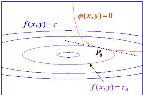
由此推知: 存在比例常数 \(\lambda_0\)，满足 \(\left( f _ { x } \left( P _ { 0 } \right) , f _ { y } \left( P _ { 0 } \right) \right) + \lambda _ { 0 } \left( \varphi _ { x } \left( P _ { 0 } \right) , \varphi _ { y } \left( P _ { 0 } \right) \right) = \left( 0 , 0 \right)\)

这又表示: 对于函数

\[ L (x, y, \lambda) = f (x, y) + \lambda \varphi (x, y), \]

在点 \(( x _ { 0 } , y _ { 0 } , \lambda _ { 0 } )\) 处恰好满足:

\[ \left. \left(f _ {x} \varphi_ {y} - f _ {y} \varphi_ {x}\right) \right| _ {P _ {0}} = 0 \]

即

\[ \left\{ \begin{array}{l} L _ {x} = f _ {x} (x, y) + \lambda \varphi_ {x} (x, y) = 0, \\ L _ {y} = f _ {y} (x, y) + \lambda \varphi_ {y} (x, y) = 0, \\ L _ {\lambda} = \varphi (x, y) = 0. \end{array} \right.\tag{2} \]

也就是说, (2) 式是函数 \(L ( x , y , \lambda )\) 在其极值点处所满足的必要条件.

由此产生了一个重要思想:

拉格朗日乘数法 对于前面定义中所设的一般目标函数和约束条件组, 应引入辅助函数

\[ \begin{array}{l} L \left(x _ {1}, x _ {2}, \dots , x _ {n}, \lambda_ {1}, \lambda_ {2}, \dots , \lambda_ {m}\right) \\ = f \left(x _ {1}, x _ {2}, \dots , x _ {n}\right) + \sum_ {k = 1} ^ {m} \lambda_ {k} \varphi_ {k} \left(x _ {1}, x _ {2}, \dots , x _ {n}\right). \end{array} \]

称此函数为拉格朗日函数, 其中 \(\lambda _ { 1 } , \lambda _ { 2 } , \cdots , \lambda _ { m }\) 称为拉格朗日乘数.

上次：含有不等式的 Constrained Optimization

The Karush–Kuhn–Tucker (KKT) Conditions

https://www.youtube.com/watch?v=uh1Dk68cfWs&t=606s （2′30″ 开始）

引入对偶变量 \(u\geq 0\)，考察 \(\max_{u\geq 0}ux\)，由此引出 Dual 与 KKT。

性质：Primal \(\geq \text{Dual}\)

原问题: \(\min _ { \boldsymbol { x } } \max _ { \lambda , \nu } L ( \boldsymbol { x } , \lambda , \nu )\) s.t. \(\lambda \geq \mathbf { 0 }\)

对偶问题: \(\begin{array} { l } { \displaystyle \max _ { \lambda , \nu } g ( \lambda , \nu ) = \max _ { \lambda , \nu } \min _ { x } L ( x , \lambda , \nu ) } \\ { \displaystyle s . t . ~ \lambda \geq 0 } \end{array}\)

\[ L (\boldsymbol {x}, \boldsymbol {\lambda}, \boldsymbol {v}) = f _ {0} (\boldsymbol {x}) + \sum \lambda_ {i} f _ {i} (\boldsymbol {x}) + \sum v _ {i} h _ {i} (\boldsymbol {x}) \]

\[ \max _ {\boldsymbol {\lambda}, \boldsymbol {v}} L (\boldsymbol {x}, \boldsymbol {\lambda}, \boldsymbol {v}) \geq L (\boldsymbol {x}, \boldsymbol {\lambda}, \boldsymbol {v}) \geq \min _ {\boldsymbol {x}} L (\boldsymbol {x}, \boldsymbol {\lambda}, \boldsymbol {v}) \]

\[ A (\boldsymbol {x}) = \max _ {\boldsymbol {\lambda}, \boldsymbol {v}} L (\boldsymbol {x}, \boldsymbol {\lambda}, \boldsymbol {v}) \geq L (\boldsymbol {x}, \boldsymbol {\lambda}, \boldsymbol {v}) \geq \min _ {\boldsymbol {x}} L (\boldsymbol {x}, \boldsymbol {\lambda}, \boldsymbol {v}) = I (\boldsymbol {\lambda}, \boldsymbol {v}) \]

\[ A (\boldsymbol {x}) \geq \min _ {\boldsymbol {x}} A (\boldsymbol {x}) \geq \max _ {\boldsymbol {\lambda}, \boldsymbol {v}} I (\boldsymbol {\lambda}, \boldsymbol {v}) \geq I (\boldsymbol {\lambda}, \boldsymbol {v}) \]

\[ P ^ {*} = \min _ {\boldsymbol {x}} A (\boldsymbol {x}) \geq \max _ {\boldsymbol {\lambda}, \boldsymbol {v}} I (\boldsymbol {\lambda}, \boldsymbol {v}) = D ^ {*} \]

KKT Conditions

Given general problem

\[ \begin{array}{c} \min _ {x \in \mathbb {R} ^ {n}} f (x) \\ \text { subject to } h _ {i} (x) \leq 0, i = 1, \ldots m \\ \ell_ {j} (x) = 0, j = 1, \ldots r \end{array} \]

The Karush–Kuhn–Tucker (KKT) conditions are:

\[ 0 \in \partial f (x) + \sum_ {i = 1} ^ {m} u _ {i} \partial h _ {i} (x) + \sum_ {j = 1} ^ {r} v _ {j} \partial \ell_ {j} (x) \]

(stationarity)

• ui · hi(x) = 0 for all i (complementary slackness)

\(h_i(x)\leq 0,\quad \ell_j(x)=0\quad\text{for all }i,j\) (primal feasibility)

\(u _ { i } \geq 0\) for all i

(dual feasibility)

例子 1

解：化成标准形式

求解

i.e.,

交换, 得

\[ \{\min _ {x} x ^ {2} \mid 1 \leq x \leq 2 \} \]

\[ \left\{\min _ {x} x ^ {2} \mid - x + 1 \leq 0 \text { and } x - 2 \leq 0 \right\} \]

\[ \min _ {x} x ^ {2} + \max _ {\lambda_ {1} \geq 0, \lambda_ {2} \geq 0} \lambda_ {1} (- x + 1) + \lambda_ {2} (x - 2) \]

\[ \min _ {x} \max _ {\lambda_ {1} \geq 0, \lambda_ {2} \geq 0} x ^ {2} + \lambda_ {1} (- x + 1) + \lambda_ {2} (x - 2) \]

\[ \max _ {\lambda_ {1} \geq 0, \lambda_ {2} \geq 0} \min _ {x} x ^ {2} + \lambda_ {1} (- x + 1) + \lambda_ {2} (x - 2) \]

由 KKT, 则

1. \(\nabla _ { x } L = 0\) ，即 \(\begin{array} { r } { 2 x - \lambda _ { 1 } + \lambda _ { 2 } = 0 \Rightarrow x ^ { \ast } = \frac { \lambda _ { 1 } - \lambda _ { 2 } } { 2 } } \end{array}\)

2. $\lambda _ { 1 } ( - x + 1 ) = 0 \qquad $ , 且 \(\lambda _ { 2 } ( x - 2 ) = 0\)

3. \(\lambda _ { 1 } \geq 0 , \lambda _ { 2 } \geq 0\)

4. \(- x + 1 \leq 0 , x - 2 \leq 0\)

由互补松弛条件（条件 2）可分为 4 种情形。因此，依题意取

\[ \left\{ \begin{array}{l l} x = 1 \\ \lambda_ {2} = 0 \end{array} \right. \Rightarrow x ^ {*} = 1. \]

例子 2

\[ \min f (x _ {1}, x _ {2}) = x _ {1} ^ {2} + 2 x _ {2} ^ {2} - 4 x _ {1} - 4 x _ {2} \]

\[ \mathsf {s . t .} \quad g _ {1} (x _ {1}, x _ {2}) = x _ {1} + x _ {2} - 3 \leq 0 \]

\[ g _ {2} \left(x _ {1}, x _ {2}\right) = 5 - x _ {1} - 2 x _ {2} \leq 0 \]

解；拉格朗日函数为：

\[ L \left(x _ {1}, x _ {2}, \lambda_ {1}, \lambda_ {2}\right) = x _ {1} ^ {2} + 2 x _ {2} ^ {2} - 4 x _ {1} - 4 x _ {2} + \lambda_ {1} \left(x _ {1} + x _ {2} - 3\right) + \lambda_ {2} \left(5 - x _ {1} - 2 x _ {2}\right) \]

对 \(x _ { 1 }\) 和 \(x _ { 2 }\) 求偏导得到的等式为：

\[ \frac {\partial L}{\partial x _ {1}} = 2 x _ {1} - 4 + \lambda_ {1} - \lambda_ {2} = 0 \]

\[ \frac {\partial L}{\partial x _ {2}} = 4 x _ {2} - 4 + \lambda_ {1} - 2 \lambda_ {2} = 0 \]

\[ \text { i.e., } \nabla f + \lambda_ {1} \nabla g _ {1} + \lambda_ {2} \nabla g _ {2} = \binom{2 x _ {1} - 4}{4 x _ {2} - 4} + \lambda_ {1} \binom{1}{1} + \lambda_ {2} \binom{- 1}{- 2} = 0 \]

另外， \(\lambda _ { i } g _ { i } = 0 ~ ( i = 1 , 2 )\) . 所以，4 个未知数，4 个方程，

注： 结合互补松弛条件 \(\lambda_i g_i=0\) 与 KKT 条件中的不等式约束，可分为以下情形：

1. 若 \(\lambda _ { 1 } = \lambda _ { 2 } = 0\) ，则 \(g _ { 1 } < 0 , g _ { 2 } < 0 ;\)

2. 若 \(\lambda _ { 1 } = 0 , \lambda _ { 2 } > 0\) ，则 \(g _ { 1 } < 0 , g _ { 2 } = 0\)

3. 若 \(\lambda _ { 1 } > 0 , \lambda _ { 2 } = 0\) ，则 \(g _ { 1 } = 0 , g _ { 2 } < 0 \colon\)

4. 若 \(\lambda _ { 1 } > 0 , \lambda _ { 2 } > 0\) ，则 \(g _ { 1 } = 0 , g _ { 2 } = 0\)

无论哪种情形，主要是求解上面写的求导后的梯度方程，即：

\[ \frac {\partial L}{\partial x _ {1}} = 2 x _ {1} - 4 + \lambda_ {1} - \lambda_ {2} = 0, \]

\[ \frac {\partial L}{\partial x _ {2}} = 4 x _ {2} - 4 + \lambda_ {1} - 2 \lambda_ {2} = 0. \]

(i) 若 \(\lambda _ { 1 } = \lambda _ { 2 } = 0\) ，则 \(g _ { 1 } < 0 , g _ { 2 } < 0\)

若 \(\lambda _ { 1 } = \lambda _ { 2 } = 0\) ，则只需要求解 \(x _ { 1 } , x _ { 2 }\) 即可：

\[ \frac {\partial L}{\partial x _ {1}} = 2 x _ {1} - 4 = 0 \Rightarrow x _ {1} = 2 \]

\[ \frac {\partial L}{\partial x _ {2}} = 4 x _ {2} - 4 = 0 \Rightarrow x _ {2} = 1 \]

那么 \(x _ { 1 } = 2 , x _ { 2 } = 1\) 就是其中的一个解了吗？

还得验证下该解是否满足不等式 \(g _ { 1 } < 0\) 和 \(g _ { 2 } < 0\)

将 \(x _ { 1 } = 2 , x _ { 2 } = 1\) 带入 \(g _ { 1 }\) 和 \(g _ { 2 }\) ，有：

\[ g _ {1} (x _ {1}, x _ {2}) = x _ {1} + x _ {2} - 3 = 2 + 1 - 3 = 0 \]

\[ g _ {2} (x _ {1}, x _ {2}) = 5 - x _ {1} - 2 x _ {2} = 5 - 2 - 2 = 1 > 0 \]

很遗憾，两个式子都无法使得 \(g _ { 1 } < 0\) 和 \(g _ { 2 } < 0\) ，故只能舍弃该解。

(ii)、(iii) 类似，我们以（iii）为例

（iii）的情形为： \(\lambda _ { 1 } > 0 , \lambda _ { 2 } = 0\) ，则 \(g _ { 1 } = 0 , g _ { 2 } < 0\)

\[ \left\{ \begin{array}{l} \frac {\partial L}{\partial x _ {1}} = 2 x _ {1} - 4 + \lambda_ {1} - \lambda_ {2} = 0 \\ \frac {\partial L}{\partial x _ {2}} = 4 x _ {2} - 4 + \lambda_ {1} - 2 \lambda_ {2} = 0 \\ g _ {1} (x _ {1}, x _ {2}) = x _ {1} + x _ {2} - 3 = 0 \\ \lambda_ {2} = 0 \end{array} \right. \Rightarrow \left\{ \begin{array}{l} x _ {1} = 2 \\ x _ {2} = 1 \\ \lambda_ {1} = 0 \\ \lambda_ {2} = 0 \end{array} \right. \]

发现此解与情形 1 的解一样（仅是这个例子一样，一般不会一样），但带入 \(g _ { 2 }\) 函数时，有：

\[ g _ {2} (x _ {1}, x _ {2}) = 5 - x _ {1} - 2 x _ {2} = 5 - 2 - 2 = 1 > 0 \]

很可惜，依然不能使得 \(g _ { 2 } < 0\) ，故该解还是需要舍弃。

(iv) 若 \(\lambda _ { 1 } > 0 , \lambda _ { 2 } > 0\) ，则 \(g _ { 1 } = 0 , g _ { 2 } = 0\)

此时，最优解在 \(g _ { 1 }\) 和 \(g _ { 2 }\) 函数的边界上，联立的四个方程为：

\[ \left\{ \begin{array}{l} \frac {\partial L}{\partial x _ {1}} = 2 x _ {1} - 4 + \lambda_ {1} - \lambda_ {2} = 0 \\ \frac {\partial L}{\partial x _ {2}} = 4 x _ {2} - 4 + \lambda_ {1} - 2 \lambda_ {2} = 0 \\ g _ {1} (x _ {1}, x _ {2}) = x _ {1} + x _ {2} - 3 = 0 \\ g _ {2} (x _ {1}, x _ {2}) = 5 - x _ {1} - 2 x _ {2} = 0 \end{array} \right. \Rightarrow \left\{ \begin{array}{l} x _ {1} = 1 \\ x _ {2} = 2 \\ \lambda_ {1} = 8 \\ \lambda_ {2} = 6 \end{array} \right. \]

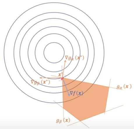
min f(x),x ∈ Rn

\(g _ { i } \left( { \pmb x } \right) = { \pmb a } _ { i } ^ { T } \cdot { \pmb x } + b _ { i } \leq 0\) 其中 \(\mathrm { i } = 1 , 2 , 3 \dots \mathrm { m } , { \pmb { a } } _ { i } \in \mathbb { R } ^ { n } , b _ { i } \in \mathbb { R }\)

\[ \begin{array}{c} L (\boldsymbol {x}, \boldsymbol {\lambda}) = f (\boldsymbol {x}) + \sum \lambda_ {i} g _ {i} \left(\boldsymbol {x}\right) \\ \Downarrow \\ \nabla L (\boldsymbol {x}, \boldsymbol {\lambda}) = 0 \\ \Downarrow \\ - \nabla f (\boldsymbol {x}) = \sum \lambda_ {i} \cdot \nabla g _ {i} \left(\boldsymbol {x}\right) \end{array} \]

KKT Conditions 的局限性

1. 必要，非充分

2. 方程可能不容易求解

上次作业: 利用 KKT conditions 求解 Optimization 问题

\[ \begin{array}{c} \min _ {x} x ^ {3} + 2 x ^ {2} - x + 1 \\ \text {s.t.} x ^ {2} \leq 1 \end{array} \]

作业解答：KKT 条件

令 \(f ( x ) = x ^ { 3 } + 2 x ^ { 2 } - x + 1 , \ g ( x ) = x ^ { 2 } - 1 \le 0\) ，可行域为 [−1,1]。拉格朗日函数为

\[ L (x, \lambda) = x ^ {3} + 2 x ^ {2} - x + 1 + \lambda (x ^ {2} - 1). \]

KKT 条件为

\[ \left\{ \begin{array}{l l} {3 x ^ {2} + 4 x - 1 + 2 \lambda x = 0,} & {\text {(驻点条件)}} \\ {x ^ {2} - 1 \leq 0,} & {\text {(原始可行性)}} \\ {\lambda \geq 0,} & {\text {(对偶可行性)}} \\ {\lambda (x ^ {2} - 1) = 0.} & {\text {(互补松弛)}} \end{array} \right. \]

作业解答：分类求解

情形一： \(| x | < 1\) （约束不活跃）。 由互补松弛得 λ = 0，因此

\[ 3 x ^ {2} + 4 x - 1 = 0 \quad \Longrightarrow \quad x = \frac {- 2 \pm \sqrt {7}}{3}. \]

其中 \(( - 2 - { \sqrt { 7 } } ) / 3 < - 1\) ，舍去；保留 \(x ^ { * } = ( - 2 + { \sqrt { 7 } } ) / 3\)

情形二： \(| x | = 1\) （约束活跃）。

\(x\)	驻点条件	结论
\(1\)	\(6+2\lambda=0\Rightarrow\lambda=-3\)	不满足 \(\lambda\geq0\)
\(-1\)	\(-2-2\lambda=0\Rightarrow\lambda=-1\)	不满足 \(\lambda\geq0\)

故唯一的 KKT 点为

\[ \boxed{(x^*,\lambda^*)=\left(\frac{\sqrt7-2}{3},0\right)}. \]

作业解答：全局最优性与最优值

f 在紧集 [−1,1] 上连续，故全局最小值必存在。所有全局极小点均满足 KKT 条件，而 KKT 点唯一，因此

\[ \boxed {x ^ {*} = \frac {\sqrt {7} - 2}{3} \approx 0.21525,} \]

\[ \boxed {f (x ^ {*}) = \frac{61-14\sqrt7}{27} \approx 0.88739} \]

也可直接验证：令 \(r = ( - 2 - { \sqrt { 7 } } ) / 3 < - 1\) ，则

\[ f ^ {\prime} (x) = 3 (x - r) \left(x - x ^ {*}\right). \]

在 \([ - 1 , x ^ { * } )\) 上 \(f ^ { \prime } ( x ) < 0\) ，在 \(( x ^ { * } , 1 ]\) 上 \(f ^ { \prime } ( x ) > 0\) ，故 f 先严格递减后严格递增， \(x ^ { * }\) 是唯一全局最优解。

注意： \(: f ^ { \prime \prime } ( x ) = 6 x + 4 \quad\) 在可行域内变号，本题不是凸优化问题；不能仅凭满足 KKT 条件就直接断言全局最优。

今天内容

Proximal Gradient 方法

Subgradient 方法

\[ \mathrm{prox} _ {\lambda f} (\pmb {v}) = \arg \min _ {\pmb {x}} (f (\pmb {x}) + \frac {1}{2 \lambda} \| \pmb {x} - \pmb {v} \| ^ {2}) \]

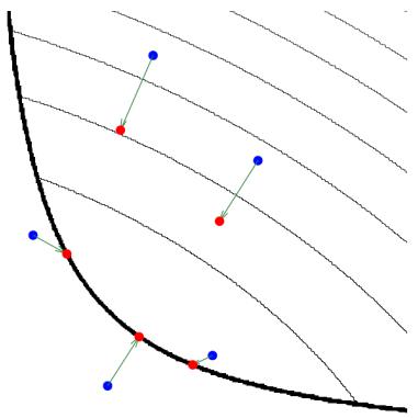
例

\[ \text { If } f = I _ {C} (\boldsymbol {x}) = \left\{ \begin{array}{l l} 0 & \boldsymbol {x} \in C \\ + \infty & \boldsymbol {x} \notin C \end{array} \right. \text { then } \]

v 在 C 上的投影

\[ \operatorname{prox} _ {f} (\boldsymbol {v}) = \arg \min _ {\boldsymbol {x} \in C} | | \boldsymbol {x} - \boldsymbol {v} | | _ {2}. \]

何时可以用 Proximal Gradient 方法？

一般的情形:

\[ \min _ {x} f (x) + g (x) \]

其中 \(f(x)\) 光滑，且 \(\operatorname{prox}_g(x)\) 易于计算时，就可采用近端梯度法。

The proximal gradient method is

\[ x ^ {k + 1} := \operatorname{prox} _ {\lambda^ {k} g} (x ^ {k} - \lambda^ {k} \nabla f (x ^ {k})),\tag{4.6} \]

where \(\lambda ^ { k } > 0\) is a step size.

什么叫 \(\operatorname{prox}_g(x)\) 容易求？

例：\(\operatorname{prox}_{\lambda f}(b)=\arg\min_x\left\{\frac{1}{2\lambda}\|x-b\|_2^2+\|x\|_1\right\}\)，其中 \(f(x)=\|x\|_1\)，且 \(x,b\) 均为标量。

解: (i) \(b \geq 0 ,\) , 显然 \(x ^ { * } \geq 0\)

\[ \text { 原式 } = \arg \min _ {x > 0} {\frac {1}{2 \lambda}} (x - b) ^ {2} + x \]

此抛物线顶点为 \(\tilde { x } = b - \lambda\)

若 \(\tilde { x } \geq 0 ,\) , 则 \(x ^ { * } = \tilde { x } = b - \lambda\) , 这时隐含着 \(b \geq \lambda\)

若 \(\tilde { x } < 0 ,\) , 则 \(x ^ { * } = 0\) , 这时 \(b < \lambda\)

所以, \(x ^ { * } = { \left\{ \begin{array} { l l } { b - \lambda } & { b \geq \lambda } \\ { 0 } & { b < \lambda } \end{array} \right. }\)

(ii) 同理, \(b < 0 ,\) 则 \(x ^ { * } = { \left\{ \begin{array} { l l } { b + \lambda } & { | b | \geq \lambda } \\ { 0 } & { | b | < \lambda } \end{array} \right. }\)

\(\phi _ { b } ( x ) = \frac { ( x - b ) ^ { 2 } } { 2 \lambda } + | x | ;\) ；取 λ = 1，横轴为 x，纵轴为函数值。

\(b = 2 > \lambda\) ：最低点在 x = 1

\[ \phi_ {2} (x) = \frac {1}{2} (x - 2) ^ {2} + | x | 。 \]

\(x \geq 0\) 时 \(\begin{array} { r } { \phi _ { 2 } ( x ) = \frac { 1 } { 2 } ( x - 1 ) ^ { 2 } + \frac { 3 } { 2 } } \end{array}\) ，故

\[ \boxed {x ^ {*} = 1, \quad \min \phi_ {2} = \frac {3}{2}} 。 \]

\(b = { \textstyle { \frac { 1 } { 2 } } } < \lambda\) ：最低点在 \(x = 0\)

\[ \phi_ {1 / 2} (x) = \frac {1}{2} (x - \frac {1}{2}) ^ {2} + | x | 。 \]

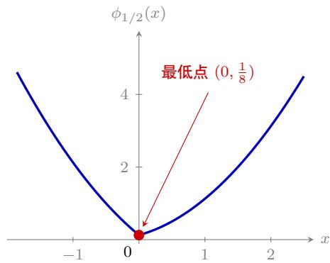
零点左导数为 \(- \frac { 3 } { 2 }\) ，右导数为 \(\frac { 1 } { 2 }\) ，故

\[ \boxed {x ^ {*} = 0, \quad \min \phi_ {1 / 2} = \frac {1}{8}}. \]

目标函数的最低点与最小值：一般结论

\[ \phi_ {b} (x) = \frac {(x - b) ^ {2}}{2 \lambda} + | x |, \quad \lambda > 0. \]

在零点两侧求导：

\[ \phi_ {b} ^ {\prime} (x) = \left\{ \begin{array}{l l} (x - b) / \lambda - 1, & x < 0, \\ (x - b) / \lambda + 1, & x > 0. \end{array} \right. \]

若 \(b > \lambda\) ，右侧驻点 \(x = b - \lambda > 0\) 是最低点；若 \(b < - \lambda\) ，左侧驻点 \(x = b + \lambda < 0\) 是最低点。 若 \(| b | \leq \lambda\) ，零点的左导数 \(- b / \lambda - 1 \leq 0\) ，右导数 \(- b / \lambda + 1 \ge 0\) ，最低点就在折点 \(x = 0\)

\[ \boxed {x ^ {*} = \operatorname{sign} (b) \max \{| b | - \lambda , 0 \},} \]

\[ \boxed {\min _ {x} \phi_ {b} (x) = \left\{ \begin{array}{l l} \frac {b ^ {2}}{2 \lambda}, & | b | \leq \lambda , \\ | b | - \frac {\lambda}{2}, & | b | > \lambda . \end{array} \right.} \]

\(\phi _ { b }\) 严格凸，因此上述最低点唯一； \(b < 0\) 的图像可由对应 \(| b |\) 的图像左右翻转得到。

\(x ^ { * } = { \left\{ \begin{array} { l l } { b - \lambda } & { b \geq \lambda } \\ { 0 } & { b < \lambda } \end{array} \right. }\) for \(b \geq 0\) 和 \(x ^ { \ast } = \left\{ { \begin{array} { l l } { b + \lambda } & { | b | \geq \lambda } \\ { 0 } & { | b | < \lambda } \end{array} } \right.\) for \(b < 0\) 可合并成

\[ x ^ {*} = \left\{ \begin{array}{l l} \operatorname{sgn} (b) (| b | - \lambda) & | b | > \lambda \\ 0 & \text { else } \end{array} \right. \tag * {\square} \]

对向量情形，若 \(f(\mathbf{x})=\|\mathbf{x}\|_1\)，则 \(\operatorname{prox}_{\lambda f}(\mathbf{b})=\arg\min_{\mathbf{x}}\left\{\frac{1}{2\lambda}\|\mathbf{x}-\mathbf{b}\|_2^2+\|\mathbf{x}\|_1\right\}\)。

\[ x _ {i} ^ {*} = \left\{ \begin{array}{l l} \operatorname{sgn} (b _ {i}) (| b _ {i} | - \lambda) & | b _ {i} | > \lambda \\ 0 & \text { else } \end{array} \right. \tag * {\square} \]

\[ \min _ {\pmb {x}} \frac {1}{2} \| A \pmb {x} - \pmb {b} \| _ {2} ^ {2} + \lambda \| \pmb {x} \| _ {1}\tag{LASSO:} \]

Subgradients

Ryan Tibshirani

Convex Optimization 10-725/36-725

回忆：gradient descent

Consider the problem

\[ \min _ {\boldsymbol {x}} f (\boldsymbol {x}) \]

for \(f\) convex and differentiable, dom \(( f ) = \mathbb { R } ^ { n }\)

Gradient descent:

choose initial \(\pmb { x } ^ { ( 0 ) } \in \mathbb { R } ^ { n }\) , repeat

\[ \boldsymbol {x} ^ {(k)} = \boldsymbol {x} ^ {(k - 1)} - t _ {k} \cdot \nabla f (\boldsymbol {x} ^ {(k - 1)}), k = 1, 2, 3, \dots \]

Step sizes \(t _ { k }\) chosen to be fixed and small, or by backtracking line search.

If ∇f Lipschitz (即 ∇f 变化不剧烈), gradient descent has convergence rate \(O ( 1 / \epsilon )\)

缺点:

Requires f differentiable

Can be slow to converge

Outline

Today: crucial mathematical underpinnings!

Subgradients

Examples

Subgradient rules

Optimality characterizations

Subgradients

Remember that for convex and differentiable \(f ,\)

\[ f (\boldsymbol {y}) \geq f (\boldsymbol {x}) + \nabla f (\boldsymbol {x}) ^ {\mathrm{T}} (\boldsymbol {y} - \boldsymbol {x}) \text { for all } \boldsymbol {x}, \boldsymbol {y} \]

i.e., linear approximation always underestimates \(f\)

A subgradient of a convex function \(f\) at \(\pmb{x}\) is any \(\pmb { g } \in \mathbb { R } ^ { n }\) such that

\[ f (\boldsymbol {y}) \geq f (\boldsymbol {x}) + \boldsymbol {g} ^ {\mathrm{T}} (\boldsymbol {y} - \boldsymbol {x}) \text { for all } \boldsymbol {y} \]

Always exists

If \(f\) is differentiable at \(x\), then \(\pmb { g } = \nabla f ( \pmb { x } )\) uniquely

Actually, same definition works for nonconvex \(f\) (however, subgradients need not exist)

Examples of subgradients

例 1. \(f : \mathbb { R } \to \mathbb { R } , f ( x ) = | x |\)

For \(x \neq 0\) , unique subgradient \(g = \operatorname{sign} \left( x \right)\)

For \(x = 0\), a subgradient \(g\) is any element of \([ - 1 , 1 ]\)

例 2. \(f : \mathbb{R}^{n} \to \mathbb{R} , f ( \pmb { x } ) = \| \pmb { x } \| _ { 2 }\)

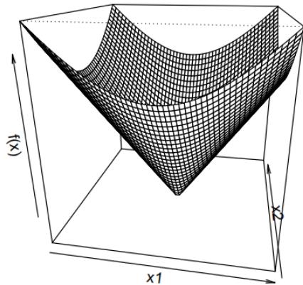
For \(\mathbf { \boldsymbol { x } } \neq \mathbf { \boldsymbol { 0 } }\) , unique subgradient \({ \pmb g } = { \pmb x } / \| { \pmb x } \| _ { 2 }\)

For \({ \pmb x } = 0\) , subgradient g is any element of \(\{ z : \| z \| _ { 2 } \leq 1 \}\)

理由：

At \(x = 0\) , the function \(f ( x ) = \| x \| _ { 2 }\) is not differentiable because the Euclidean norm has a "sharp" point at the origin (like a cone vertex). In this case, the subgradient is defined as any vector \(g\) that satisfies the subgradient inequality:

\[ f (y) \geq f (0) + g ^ {\top} (y - 0), \quad \forall y \in \mathbb {R} ^ {n}. \]

Since \(f ( 0 ) = 0 ,\) , this simplifies to:

\[ \| y \| _ {2} \geq g ^ {\top} y, \quad \forall y \in \mathbb {R} ^ {n}. \]

The inequality \(g ^ { \top } y \leq \| y \| _ { 2 }\) holds if and only if g satisfies \(\| g \| _ { 2 } \leq 1\) . Therefore, the subgradient set at \(x=0\) is

\[ \{z \in \mathbb {R} ^ {n}: \| z \| _ {2} \leq 1 \}. \]

This includes all vectors within or on the surface of the unit ball in \(\mathbb { R } ^ { n }\)

例 3. \(f : \mathbb{R}^{n} \to \mathbb{R} , f ( \pmb { x } ) = \| \pmb { x } \| _ { 1 }\)

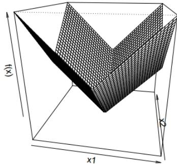
For \(x _ { i } \neq 0\) , unique ith component \(g _ { i } = \operatorname{sign} ( x _ { i } )\)

For \(x_i=0\), the \(i\)th component \(g _ { i }\) is any element of \([ - 1 , 1 ]\)

例 4. Let \(f _ { 1 } , f _ { 2 } : \mathbb{R}^{n} \to \mathbb{R}\) be convex and differentiable, and \(f ( \pmb { x } ) = \max \{ f _ { 1 } ( \pmb { x } ) , f _ { 2 } ( \pmb { x } ) \}\)

For \(f _ { 1 } ( { \pmb x } ) > f _ { 2 } ( { \pmb x } )\) , unique subgradient \(\pmb { g } = \nabla f _ { 1 } ( \pmb { x } )\)

For \(f _ { 2 } ( { \pmb x } ) > f _ { 1 } ( { \pmb x } )\) , unique subgradient \({ \pmb g } = \nabla f _ { 2 } ( { \pmb x } )\)

For \(f _ { 1 } ( { \pmb x } ) = f _ { 2 } ( { \pmb x } )\) , subgradient g is any point on the line segment between \(\nabla f _ { 1 } ( { \pmb x } )\) and \(\nabla f _ { 2 } ( { \pmb x } )\)

Subdifferential

Set of all subgradients of convex \(f\) is called the subdifferential:

\(\partial f(\pmb{x})=\{\pmb{g}\in\mathbb{R}^{n}: g \text{ is a subgradient of }f\text{ at }\pmb{x}\}\)

\(\partial f ( { \pmb x } )\) is closed and convex (even for nonconvex \(f )\)

Nonempty (can be empty for nonconvex \(f )\)

If \(f\) is differentiable at x, then \(\partial f ( { \pmb x } ) = \{ \nabla f ( { \pmb x } ) \}\)

If \(\partial f ( { \pmb x } ) = \{ { \pmb g } \}\) , then \(f\) is differentiable at x and \(\nabla f ( { \pmb x } ) = { \pmb g }\)

Connection to convex geometry

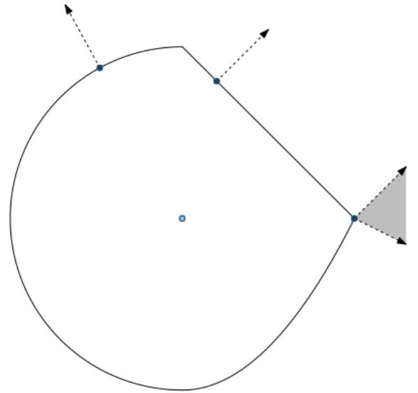
Convex set \(C \subseteq \mathbb { R } ^ { n }\) , consider the indicator function \(I_C:\mathbb{R}^n\to\mathbb{R}\cup\{+\infty\}\)

\[ I _ {C} (\boldsymbol {x}) = I \{\boldsymbol {x} \in C \} = \left\{ \begin{array}{l l} 0 & i f \boldsymbol {x} \in C \\ \infty & i f \boldsymbol {x} \notin C \end{array} \right. \]

For \(\pmb{x}\in C\), \(\partial I_C(\pmb{x})=\mathcal{N}_C(\pmb{x})\), the normal cone of \(C\) at \(\pmb{x}\). Recall

\[ \mathcal {N} _ {C} (\boldsymbol {x}) = \left\{\boldsymbol {g} \in \mathbb {R} ^ {n}: \boldsymbol {g} ^ {\mathrm{T}} \boldsymbol {x} \geq \boldsymbol {g} ^ {\mathrm{T}} \boldsymbol {y} \text { for any } \boldsymbol {y} \in C \right\} \]

Why? By definition of a subgradient \(\pmb{g}\),

\[ I _ {C} (\boldsymbol {y}) \geq I _ {C} (\boldsymbol {x}) + \boldsymbol {g} ^ {T} (\boldsymbol {y} - \boldsymbol {x}) \text { for all } \boldsymbol {y} \]

For \(\pmb { y } \notin C , I _ { C } ( \pmb { y } ) = \infty\)

For \(\pmb { y } \in C\) , this means \(0 \geq \pmb { g } ^ { T } ( \pmb { y } - \pmb { x } )\)

Subgradient calculus

Basic rules for convex functions:

Scaling: \(\partial ( a f ) = a \cdot \partial f\) provided \(a > 0\)

Addition: \(\partial ( f _ { 1 } + f _ { 2 } ) = \partial f _ { 1 } + \partial f _ { 2 }\)

Affine composition: if \(g ( { \pmb x } ) = f ( A { \pmb x } + { \pmb b } )\) , then

\[ \partial g (\boldsymbol {x}) = A ^ {\mathrm{T}} \partial f (A \boldsymbol {x} + \boldsymbol {b}) \]

Finite pointwise maximum: if \(f ( \pmb { x } ) = \max _ { i = 1 , \dots m } f _ { i } ( \pmb { x } )\) , then

\[ \partial f (\boldsymbol {x}) = \operatorname{conv} \left(\bigcup_ {i: f _ {i} (\boldsymbol {x}) = f (\boldsymbol {x})} \partial f _ {i} (\boldsymbol {x})\right) \]

the convex hull of union of subdifferentials of all active functions at x

General pointwise maximum: if \(f ( \pmb { x } ) = \max _ { s \in S } f _ { s } ( \pmb { x } )\) , then

\[ \partial f (\boldsymbol {x}) \supseteq \operatorname{cl} \left\{\operatorname{conv} \left(\bigcup_ {s: f _ {s} (\boldsymbol {x}) = f (\boldsymbol {x})} \partial f _ {s} (\boldsymbol {x})\right) \right\} \]

and under some regularity conditions (on \(S , f _ { s } )\) , we get an equality above

Norms: important special case, \(f ( \pmb { x } ) = \| \pmb { x } \| _ { p }\) . Let \(q\) be such that \(1 / p + 1 / q = 1\) , then

\[ \| \boldsymbol {x} \| _ {p} = \max _ {\| \boldsymbol {z} \| _ {q} \leq 1} \boldsymbol {z} ^ {\mathrm{T}} \boldsymbol {x} \]

Hence

\[ \partial f (\boldsymbol {x}) = \operatorname{argmax} _ {\| \boldsymbol {z} \| _ {q} \leq 1} z ^ {\mathrm{T}} \boldsymbol {x} \]

Why subgradients?

Subgradients are important for two reasons:

Convex analysis: optimality characterization via subgradients, monotonicity, relationship to duality

Convex optimization: if you can compute subgradients, then you can minimize (almost) any convex function

Optimality condition

For any f (convex or not),

\[ f (\boldsymbol {x} ^ {\star}) = \min _ {\boldsymbol {x}} f (\boldsymbol {x}) \Longleftrightarrow \mathbf {0} \in \partial f (\boldsymbol {x} ^ {\star}) \]

i.e., \({ \pmb x } ^ { \star }\) is a minimizer if and only if 0 is a subgradient of \(f\) at \({ \pmb x } ^ { \star }\) .

This is called the subgradient optimality condition

Why? Easy: \(\mathbf { \nabla } _ { \mathbf { \pmb { g } } } = \mathbf { 0 }\) being a subgradient means that for all \(\textbf { { y } }\)

\[ f (\boldsymbol {y}) \geq f (\boldsymbol {x} ^ {\star}) + \mathbf {0} ^ {\mathrm{T}} (\boldsymbol {y} - \boldsymbol {x} ^ {\star}) = f (\boldsymbol {x} ^ {\star}) \]

Note the implication for a convex and differentiable function \(f ,\) , with \(\partial f ( { \pmb x } ) = \{ \nabla f ( { \pmb x } ) \}\)

Derivation of first-order optimality

Example of the power of subgradients: we can use what we have learned so far to derive the first-order optimality condition.

Recall that for \(f\) convex and differentiable, the problem

\[ \min _ {\boldsymbol {x}} f (\boldsymbol {x}) \text { subject to } \boldsymbol {x} \in C \]

is solved at x if and only if

\[ \nabla f (\boldsymbol {x}) ^ {\mathrm{T}} (\boldsymbol {y} - \boldsymbol {x}) \geq 0 \text { for all } \boldsymbol {y} \in C \]

Intuitively, this says that the gradient points toward increasing function values as we move away from \(x\). How to see this? First recast problem as min f(x) + I_C(x)

\[ \min _ {\boldsymbol {x}} f (\boldsymbol {x}) + I _ {C} (\boldsymbol {x}) \]

Now apply subgradient optimality: \({ \bf 0 } \in \partial ( f ( { \pmb x } ) + I _ { C } ( { \pmb x } ) )\)

But

\[ \begin{array}{l} \mathbf {0} \in \partial (f (\boldsymbol {x}) + I _ {C} (\boldsymbol {x})) \\ \Longleftrightarrow \mathbf {0} \in \{\nabla f (\boldsymbol {x}) \} + \mathcal {N} _ {C} (\boldsymbol {x}) \\ \Longleftrightarrow - \nabla f (\boldsymbol {x}) \in \mathcal {N} _ {C} (\boldsymbol {x}) \\ \Longleftrightarrow - \nabla f (\boldsymbol {x}) ^ {\mathrm{T}} \boldsymbol {x} \geq - \nabla f (\boldsymbol {x}) ^ {\mathrm{T}} \boldsymbol {y} \text {for all} \boldsymbol {y} \in C \\ \Longleftrightarrow \nabla f (\boldsymbol {x}) ^ {\mathrm{T}} (\boldsymbol {y} - \boldsymbol {x}) \geq 0 \text {for all} \boldsymbol {y} \in C \end{array} \]

as desired

Note: the condition \({ \bf 0 } \in \partial f ( { \pmb x } ) + \mathcal { N } _ { C } ( { \pmb x } )\) is a fully general condition for optimality in a convex problem. But this is not always easy to work with (KKT conditions, later, are easier)

Example: lasso (least absolute shrinkage and selection operator) optimality conditions

Given \(\pmb { y } \in \mathbb { R } ^ { n } , X \in \mathbb { R } ^ { n \times p }\) , lasso problem can be parametrized as:

\[ \min _ {\boldsymbol {\beta} \in \mathbb {R} ^ {p}} \frac {1}{2} \| \boldsymbol {y} - X \boldsymbol {\beta} \| _ {2} ^ {2} + \lambda \| \boldsymbol {\beta} \| _ {1} \]

where \(\lambda \geq 0\) . Subgradient optimality:

\[ \begin{array}{l} \mathbf {0} \in \partial \left(\frac {1}{2} \| \boldsymbol {y} - X \boldsymbol {\beta} \| _ {2} ^ {2} + \lambda \| \boldsymbol {\beta} \| _ {1}\right) \\ \Longleftrightarrow \mathbf {0} \in - X ^ {\mathrm{T}} (\boldsymbol {y} - X \boldsymbol {\beta}) + \lambda \partial \| \boldsymbol {\beta} \| _ {1} \\ \Longleftrightarrow X ^ {\mathrm{T}} (\boldsymbol {y} - X \boldsymbol {\beta}) = \lambda \boldsymbol {v} \end{array} \]

for some \({ \pmb v } \in \partial \| \beta \| _ { 1 }\) , i.e.,

\[ \boldsymbol {v} _ {i} \in \left\{ \begin{array}{l l} \{1 \} & \text {if} \beta_ {i} > 0 \\ \{- 1 \} & \text {if} \beta_ {i} < 0, i = 1, \ldots , p \\ [ - 1, 1 ] & \text {if} \beta_ {i} = 0 \end{array} \right. \]

Write \(\pmb { x } _ { 1 } , \cdots , \pmb { x } _ { p }\) for columns of X. Then subgradient optimality reads:

\[ \left\{ \begin{array}{r l} \boldsymbol {x} _ {i} ^ {\mathrm{T}} (\boldsymbol {y} - X \boldsymbol {\beta}) = \lambda \cdot \operatorname{sign} (\beta_ {i}) & \text {if} \beta_ {i} \neq 0 \\ | \boldsymbol {x} _ {i} ^ {\mathrm{T}} (\boldsymbol {y} - X \boldsymbol {\beta}) | \leq \lambda & \text {if} \beta_ {i} = 0 \end{array} \right. \]

Note: The subgradient optimality conditions do not directly give a lasso solution, but they do provide a way to check lasso optimality.

They are also helpful in understanding the lasso estimator; e.g., if

\(| { \pmb x } _ { i } ^ { \mathrm { T } } ( { \pmb y } - X { \pmb \beta } ) | < \lambda\) , then \(\beta _ { i } = 0\)

Example: soft-thresholding

Simplified lasso problem with \(X = I !\)

\[ \min _ {\boldsymbol {\beta} \in \mathbb {R} ^ {n}} \frac {1}{2} \| \boldsymbol {y} - \boldsymbol {\beta} \| _ {2} ^ {2} + \lambda \| \boldsymbol {\beta} \| _ {1} \]

This we can solve directly using subgradient optimality. Solution is \(\beta = S _ { \lambda } ( \pmb { y } )\) , where \(S _ { \lambda }\) is the soft-thresholding operator:

\[ [ S _ {\lambda} (\boldsymbol {y}) ] _ {i} = \left\{ \begin{array}{l l} y _ {i} - \lambda & i f \quad y _ {i} > \lambda \\ 0 & i f \quad - \lambda \leq y _ {i} \leq \lambda , i = 1, \dots n \\ y _ {i} + \lambda & i f \quad y _ {i} < - \lambda \end{array} \right. \]

Check: from last slide, subgradient optimality conditions are

\[ \left\{ \begin{array}{r l} y _ {i} - \beta_ {i} = \lambda \cdot \mathrm{sign} (\beta_ {i}) & i f \beta_ {i} \neq 0 \\ | y _ {i} - \beta_ {i} | \leq \lambda & i f \beta_ {i} = 0 \end{array} \right. \]

Now plug in \(\beta = S _ { \lambda } ( \pmb { y } )\) and check these are satisfied:

When \(y _ { i } > \lambda , \beta _ { i } = y _ { i } - \lambda > 0\) , so \(y _ { i } - \beta _ { i } = \lambda = \lambda \cdot 1\)

When \(y _ { i } < - \lambda\) , argument is similar

When \(| y _ { i } | \leq \lambda , \beta _ { i } = 0\) , and \(| y _ { i } - \beta _ { i } | = | y _ { i } | \leq \lambda\)

Soft-thresholding in one variable:

近端梯度法的应用：稀疏信号去噪

测得信号 \(\pmb { b } = ( 3 , 0 . 2 , - 2 ) ^ { \top }\) ，希望去掉小噪声，保留主要信号。假设真实信号应当稀疏，建立模型

\[ \min _ {\pmb {x} \in \mathbb {R} ^ {3}} F (\pmb {x}) = \underbrace {\frac {1}{2} \| \pmb {x} - \pmb {b} \| _ {2} ^ {2}} _ {\text {贴近观测}} + \underbrace {\| \pmb {x} \| _ {1}} _ {\text {鼓励零分量}}. \]

这是 LASSO 的特例： \(A = I\) ，正则化参数 \(\lambda = 1\)

\[ f (\boldsymbol {x}) = \frac {1}{2} \| \boldsymbol {x} - \boldsymbol {b} \| _ {2} ^ {2}, \qquad h (\boldsymbol {x}) = \| \boldsymbol {x} \| _ {1}, \qquad \nabla f (\boldsymbol {x}) = \boldsymbol {x} - \boldsymbol {b} \]

选择步长 t = 1，使用近端梯度更新

\[ \boldsymbol {x} ^ {k + 1} = \operatorname{prox} _ {t h} \left(\boldsymbol {x} ^ {k} - t \nabla f (\boldsymbol {x} ^ {k})\right). \]

近端梯度法的应用：一步算出答案

第一步：梯度步。任意初始点 \(x ^ { 0 }\) 都有

\[ \boldsymbol {v} = \boldsymbol {x} ^ {0} - (\boldsymbol {x} ^ {0} - \boldsymbol {b}) = \boldsymbol {b} = (3, 0.2, - 2) ^ {\top}. \]

第二步：近端步。逐坐标应用阈值为 1 的软阈值算子：

\[ S _ {1} (u) = \operatorname{sign} (u) \max \{| u | - 1, 0 \}. \]

\[ 3 \longmapsto 2, \qquad 0.2 \longmapsto 0, \qquad - 2 \longmapsto - 1. \]

\[ \boxed {x ^ {*} = S _ {1} (b) = (2, 0, - 1) ^ {\mathsf {T}}.} \]

解释：小分量 0.2 被置零，大分量向零收缩 1。这里一步求解来自 A = I 和 t = 1 的特殊结构；一般LASSO 需要迭代。

次梯度法的应用：用绝对误差寻找代表值

有三个观测值 \(1,3,8\)，希望找一个数 \(x\) 代表它们，最小化总绝对误差：

\[ \min _ {x \in \mathbb {R}} F (x) = | x - 1 | + | x - 3 | + | x - 8 |. \]

绝对值在零点不可微，采用次梯度法。对单项有

\[ \partial | x - a | = \left\{ \begin{array}{l l} \{- 1 \}, & x < a, \\ [ - 1, 1 ], & x = a, \\ \{1 \}, & x > a. \end{array} \right. \]

取 \(\operatorname{sign} ( 0 ) = 0\) ，可选次梯度

\[ g (x) = \operatorname{sign} (x - 1) + \operatorname{sign} (x - 3) + \operatorname{sign} (x - 8) \in \partial F (x). \]

更新公式为 \(\boxed { x ^ { k + 1 } = x ^ { k } - \alpha _ { k } g ( x ^ { k } ) }\)

次梯度法的应用：手算迭代过程

从 \(x ^ { 0 } = 6\) 出发，本例取固定步长 \(\alpha _ { k } = 1\)

\[ \begin{array}{c c c c} k & x ^ {k} & g (x ^ {k}) & F (x ^ {k}) \\ \hline 0 & 6 & 1 + 1 - 1 = 1 & 10 \\ 1 & 5 & 1 + 1 - 1 = 1 & 9 \\ 2 & 4 & 1 + 1 - 1 = 1 & 8 \\ 3 & 3 & 1 + 0 - 1 = 0 & 7 \end{array} \]

\[ 6 \longrightarrow 5 \longrightarrow 4 \longrightarrow \boxed {3}. \]

由于 F 凸且 \(0 \in \partial F ( 3 ) , x ^ { * } = 3\) 是全局最优解。它也是三个观测值的中位数， \(\boxed { F ( x ^ { * } ) = 7 }\) 注意：这里恰好有限步到达最优点；一般问题用固定步长可能振荡。常用递减步长，例如 \(\alpha _ { k } = c / ( k + 1 )\) \(\left( c > 0 \right)\)

两种方法：这两个例子说明了什么？

近端梯度法：将目标写为 F = f +h，对光滑项 f 作梯度步，再精确求解包含非光滑项 h 的近端子问题：

\[ x ^ {k + 1} = \arg \min _ {z} \left\{h (z) + \frac {1}{2 t} \| z - (x ^ {k} - t \nabla f (x ^ {k})) \| _ {2} ^ {2} \right\}. \]

稀疏去噪例子中，近端子问题可直接用软阈值公式求解。

次梯度法：选取整个凸目标函数的一个次梯度，直接更新：

\[ g ^ {k} \in \partial F (x ^ {k}), \qquad x ^ {k + 1} = x ^ {k} - \alpha_ {k} g ^ {k}. \]

绝对误差例子中，只需计算三个符号函数的和。

选择依据：近端映射容易计算时适合使用近端梯度法；次梯度容易计算时，可以使用次梯度法，但需注意步长与收敛速度。